I recently fell down a very deep monochrome-shaped rabbit hole during my search for a cartographic style for this website. Part of that rabbit hole fascinated me immensely — hachure maps.

The short description of hachures is that they are a method of displaying relief on a map using nothing but lines of varying thickness. They’ve been around for a long time and are a great way to represent detail on terrain, especially in an era when printing technology was limited.

This tutorial is the result of a couple days of experimentation in QGIS on how to replicate the hachure style using geometry generators and other new features inside the latest QGIS 3.20 release.

I’ve tried to keep things as simple as possible, though I’ve also gone into as much detail as possible. It’s worth mentioning that I’ve diverged from the traditional definition of hachures, though this approach is similar enough to fit the term.

---

I’d like to thank Benjamin Becquet who helped point me in the right direction on Twitter when I first started asking about hachure styling in QGIS. Definitely check out his feed as he’s also working on similar cartographic styles.

---

Locate your area of interest

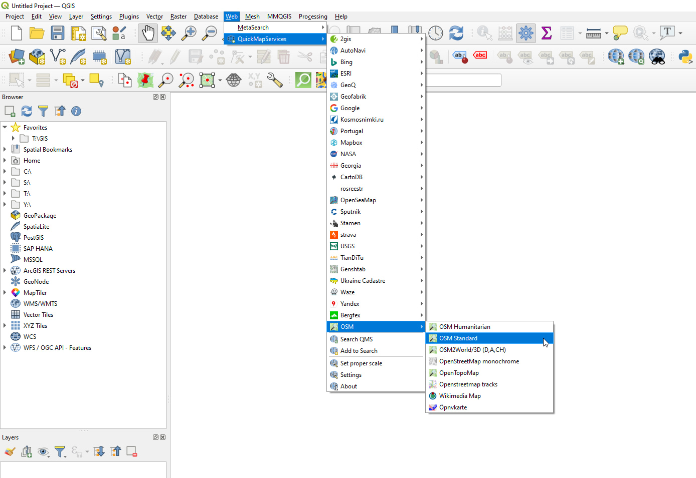
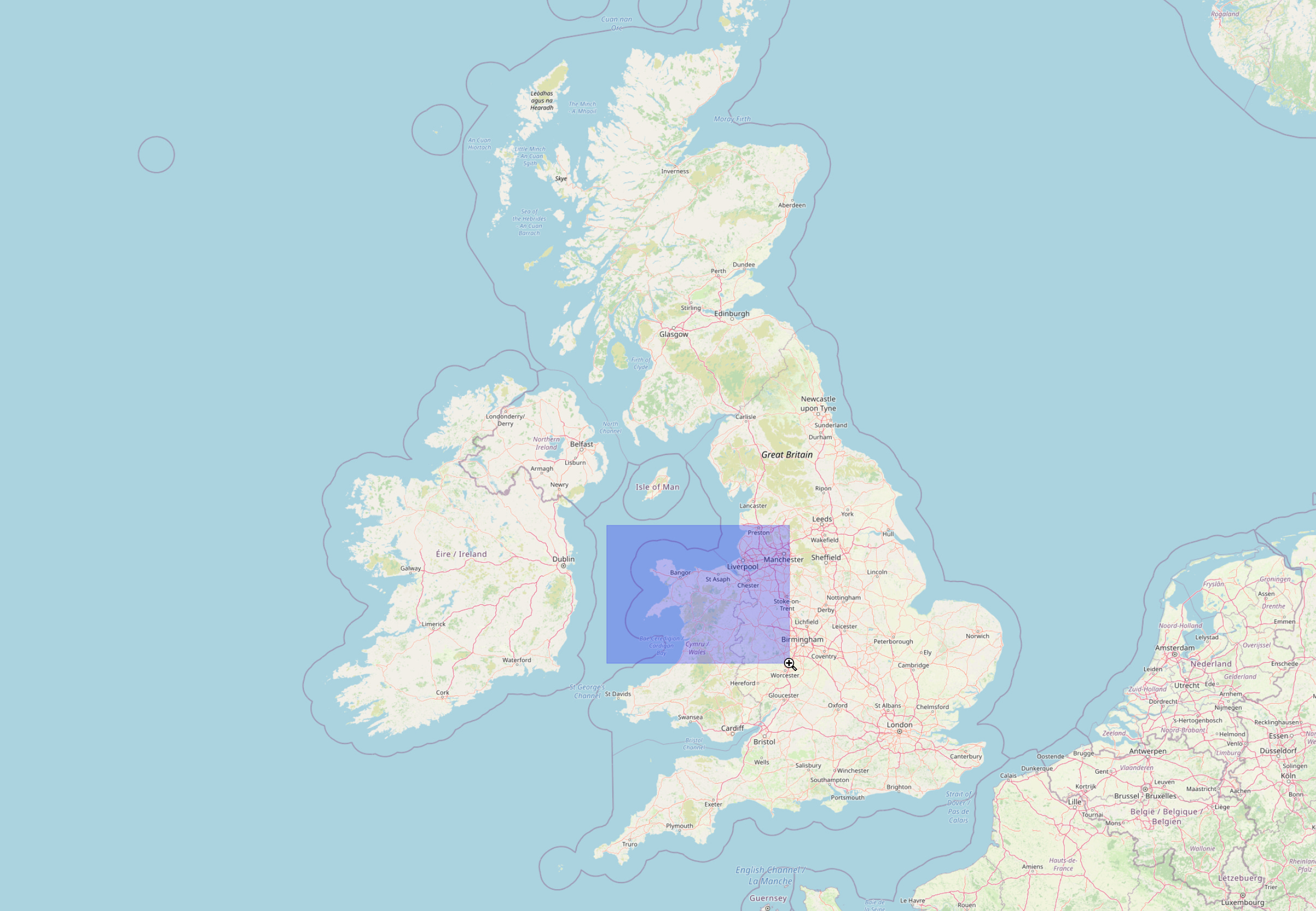
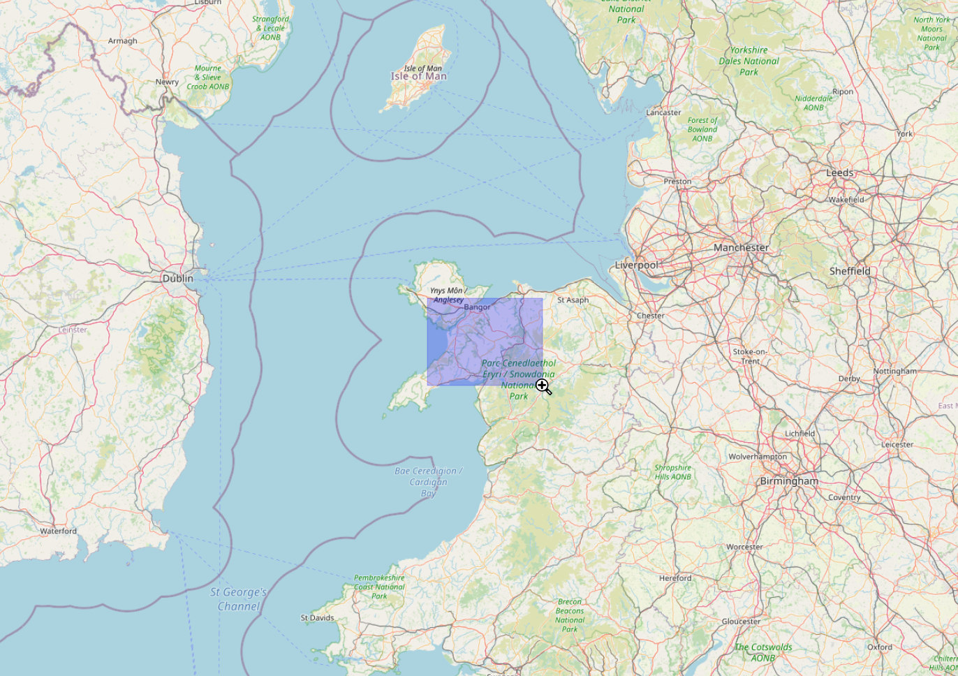
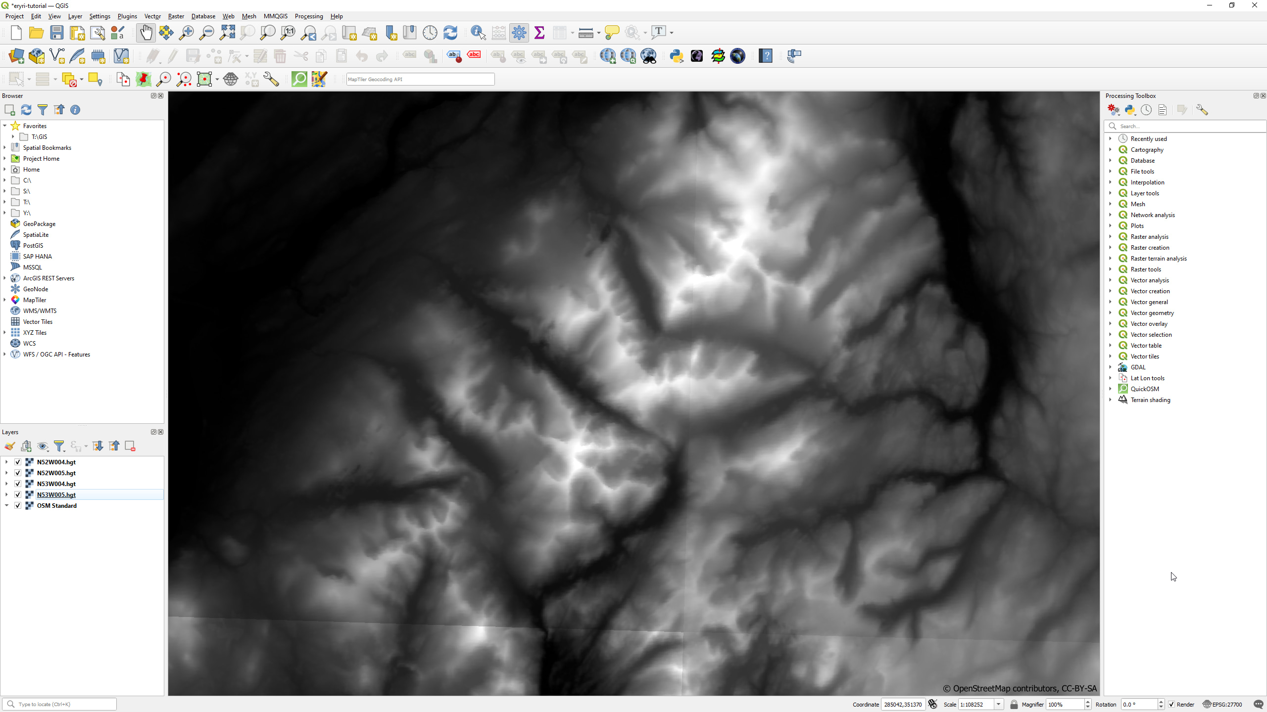
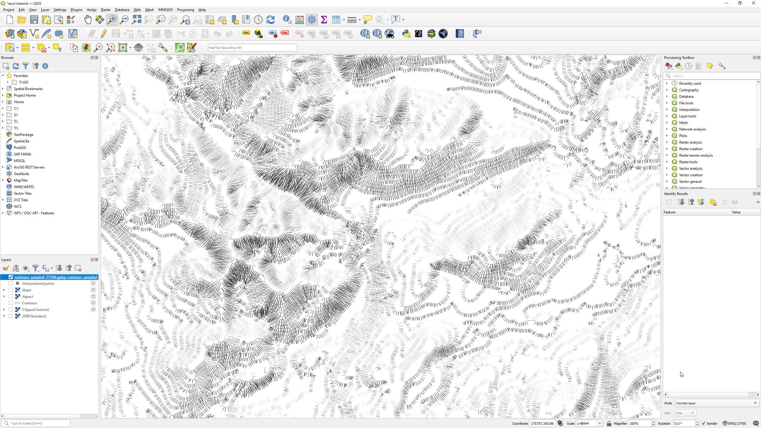
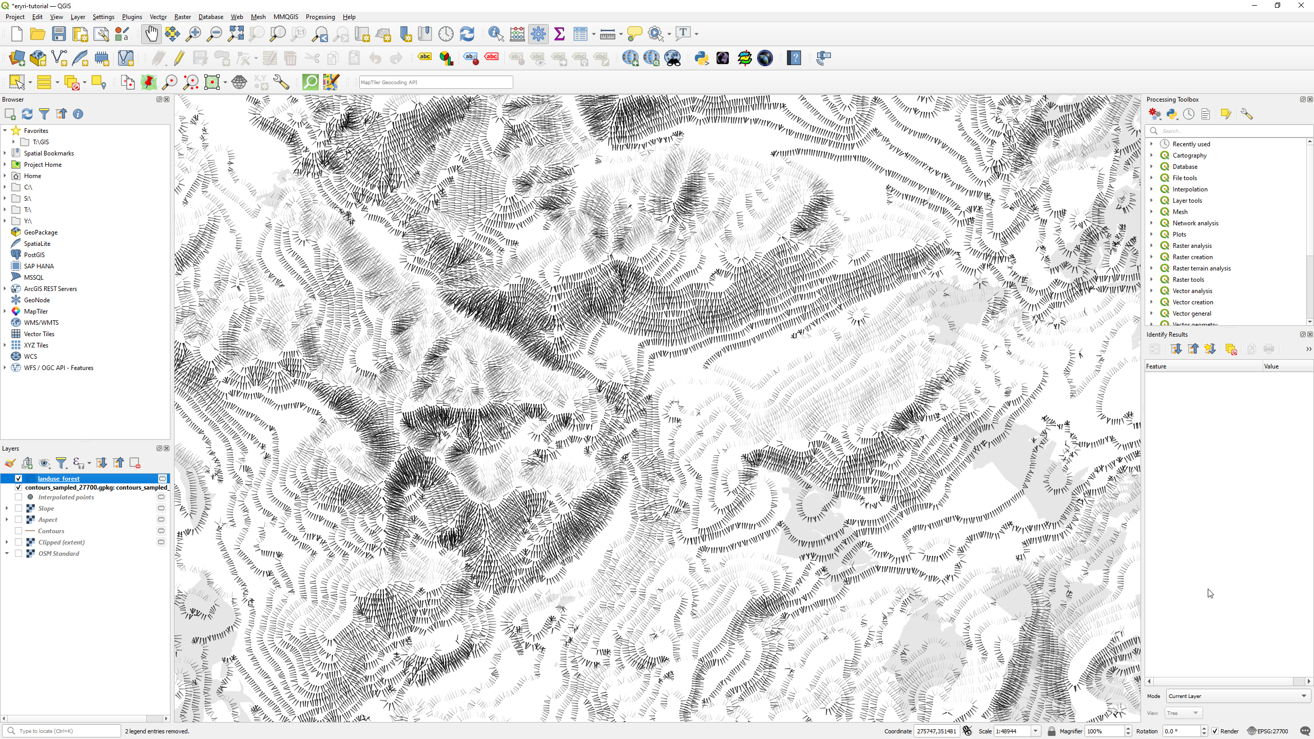
The first step is to set up your QGIS canvas with the location you want to generate the hachure map for. There are multiple ways to do this but I find it easiest to load in a basemap using the QuickMapServices plugin and using that to zoom in.

For this tutorial I’ve chosen Eryri (Snowdonia) in North Wales for no other reason than it being local to me and that I adore it. Feel free to select your own location, though bear in mind that hachures look best in more rugged areas.

Select a metric projection

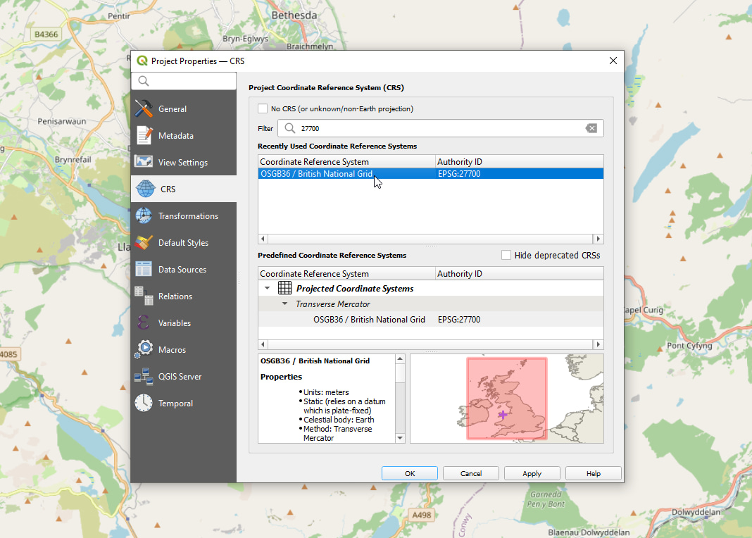
Once you have a location it’s time to select a metric projection. This is required for a couple of reasons, though it’s mostly to ensure that horizontal units are in a 1:1 ratio and both horizontal and vertical units are in metres.

If you’re also using Eryri then you can set this to the Ordnance Survey British National Grid (EPSG:27700), otherwise select another projection that’s appropriate for your chosen location.

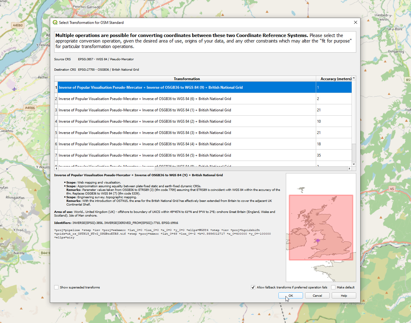
You may be asked to select a transformation method depending on the projection you’re using — in my case I selected the default option but you may need to pick something different. This is for reprojecting the Spherical Mercator basemap, which we’re only using for reference so we don’t need to be too precise here.

Save your project (often)

While QGIS is great, I’ve had plenty of prior experience of it crashing on me without warning. With that in mind I highly recommend you save early and save often when working within it.

Either press Ctrl + S or select the save option via the Project → Save menu. Give the project a name and place it somewhere you’ll be able to find it — I suggest putting it in a directory of its own as we’ll be adding a few files to it later on.

Download the SRTM DEM

We’ll be utilising DEM / elevation data throughout this tutorial so let’s go grab that now. There are many sources for elevation data, though we’ll be using the nifty SRTM Downloader plugin to save some time.

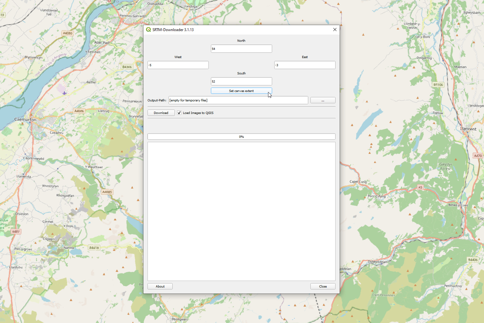
Make sure the QGIS map canvas is roughly showing the area you want to work with and then click on the SRTM Downloader icon — the black circle with a view of the Earth from space.

Click Set canvas extent to ensure that we only download the data we need, and then select a directory to store the elevation tiles (I suggest the one you just saved the project).

Click download and then one of two things will happen:

• If you’ve already used this plugin then the tiles will download and appear on the map
• If you haven’t used the plugin you’ll be asked for a username and password, in which case you’ll need to follow the link to register and then come back here

---

If you have trouble using the SRTM Downloader plugin then you can pull in elevation data from another source. An alternative method for SRTM data is Derek Watkins’ SRTM Tiler Downloader website.

---

Once the download is completed you might get a warning about transformations again — so select the appropriate one or ignore it — and you’ll see the elevation data appear on the map.

You may have already noticed the lines across the elevation output at the tile boundaries. We’ll sort this out now by creating a virtual raster file:

• Select Raster → Miscellaneous → Build Virtual Raster... from the menu
• Click the ... button next to input layers and select the elevation tiles
• If you want to save the virtual raster you can scroll down to select a location, otherwise it will be added as a temporary layer
• Click the Run button

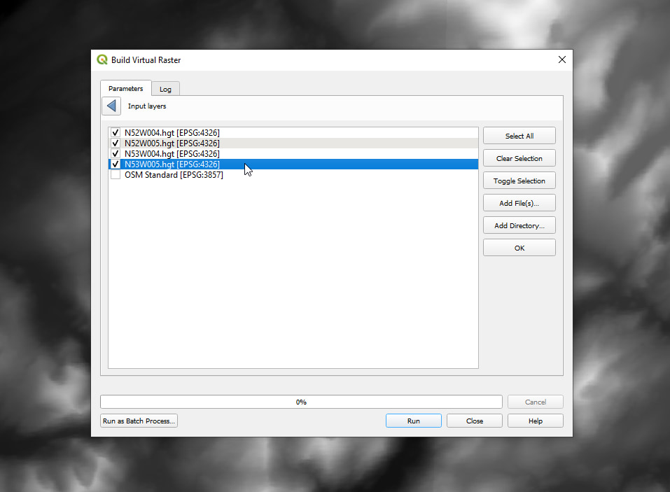
If everything worked then you’ll see a Virtual layer in the layers list — you may need to hide the other elevation layers to see it. If you want to keep things tidy then you can remove the old elevation layers now, though still keep the files as the virtual raster references them.

Transform DEM into the metric projection

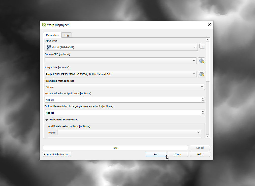
If you used SRTM then the elevation data is currently using WGS84 and needs to be transformed into the same metric system that you’re using elsewhere:

• Select Raster → Projections → Warp (Reproject)... from the menu
• Make sure the clipped elevation layer is selected as input
• Set the target CRS to the same system you used before (eg. EPSG:27700)
• Select Bilinear as the resampling method

You’ll see a new layer that contains the elevation data in the correct projection. Feel free to remove the virtual raster layer if you want as we don’t need it anymore.

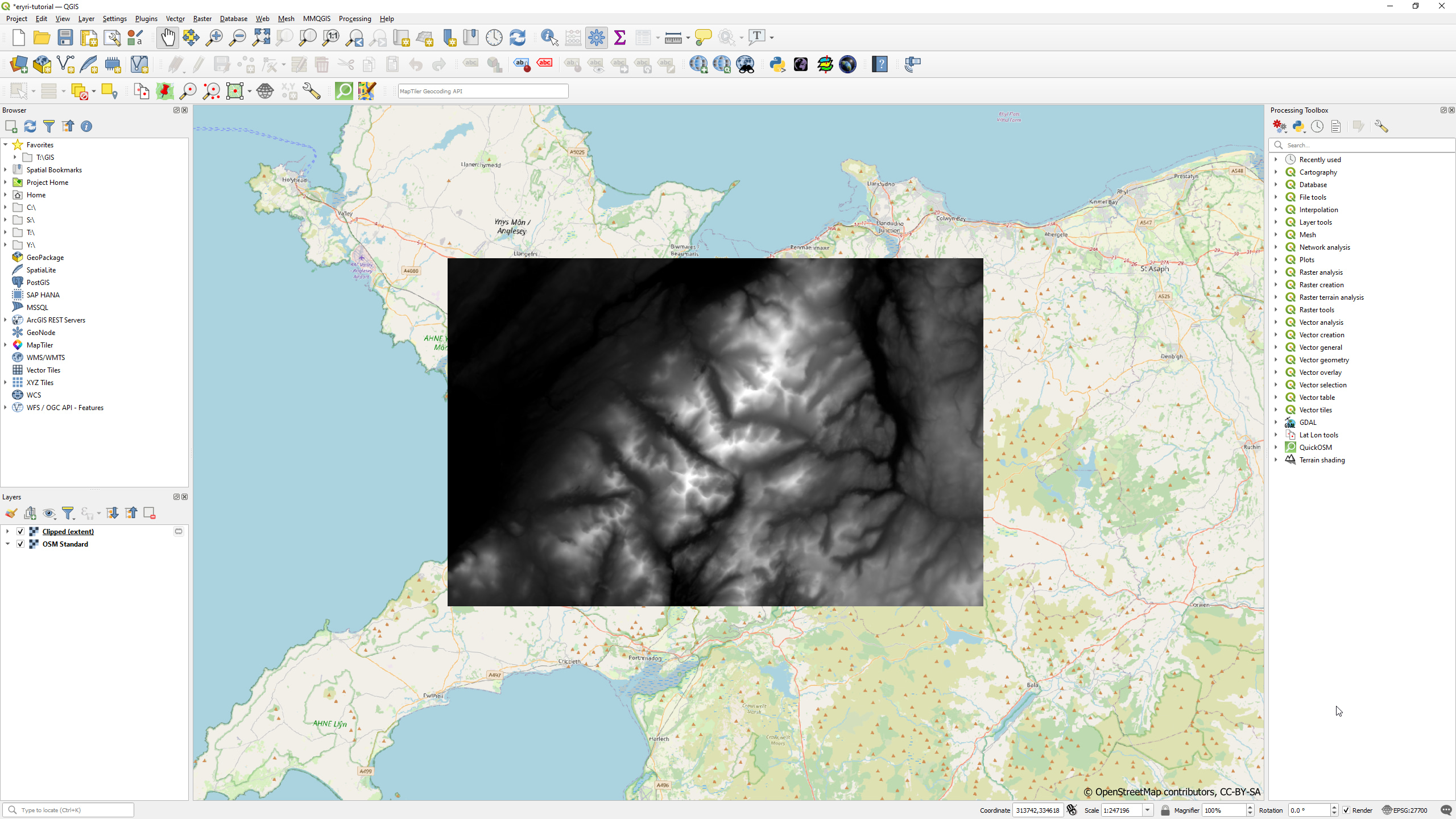
Clip the DEM to the area of interest

Right now the DEM is probably much larger than the extent of your map canvas as the SRTM tiles cover a very large area. This can add a lot of extra processing as we move on so let’s clip this to the specific area we’re interested in.

• Open up the clipping tool by selecting Raster → Extraction → Clip Raster by Extent... from the menu
• Make sure the projected raster is selected at the input layer
• Set the clipping extent to Use Map Canvas Extent
• If you want to save the clipped extent you can scroll down to select a location, otherwise it will be added as a temporary layer
• Click the Run button

You won’t immediately notice anything different, though a new elevation layer will have been added which is now clipped to the extent of the map canvas. If you zoom the map out a little you’ll notice that the elevation raster has been clipped.

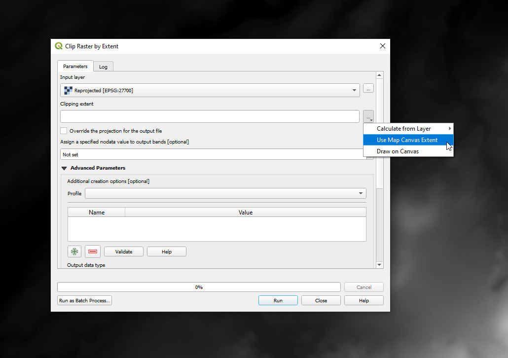
The projected raster layer can be removed as we won’t be using it anymore.

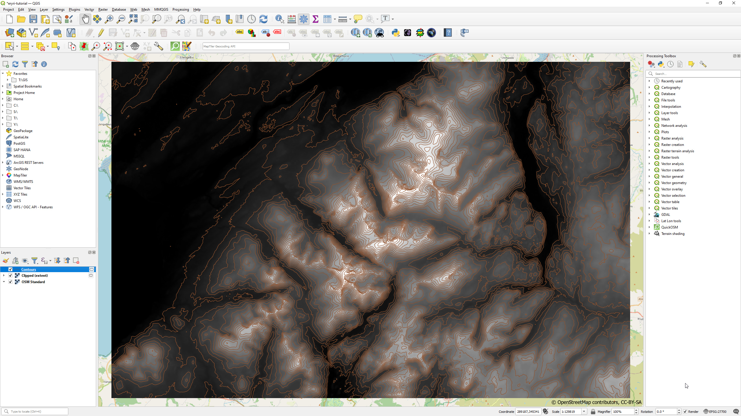
Generate the contours

Now we can make some big steps towards the hachures, starting with generating contours from the elevation data.

• Select Raster → Extraction → Contour... from the menu
• Set the interval to a value that makes sense for your location and is a balance between too sparse and too detailed (I used 50 metres)
• Click the Run button

You may have to wait for a little while depending on the size of your location and the specs of your computer, though you’ll eventually see a new contour layer appear on the map.

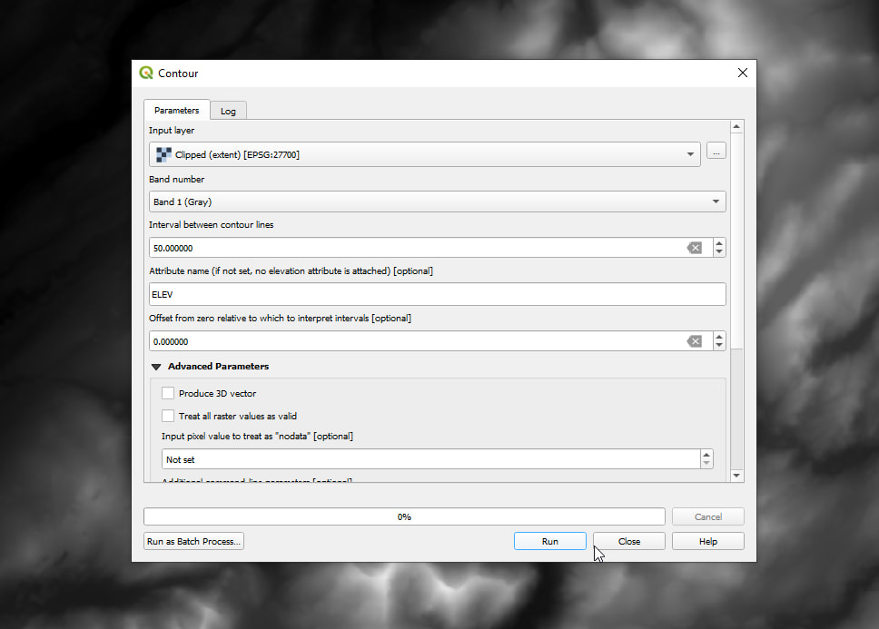
We’ll be using these contours as the basis for the hachure lines, though there are still a few more steps before we get to that.

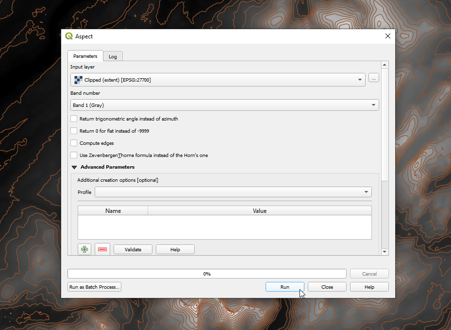
Generate the aspect and slope rasters

There are two remaining components that are required for us to generate the hachure lines — slope and aspect. We’ll be using these to work out the steepness and orientation of the elevation data, which will dramatically improve the visual fidelity of the hachure lines.

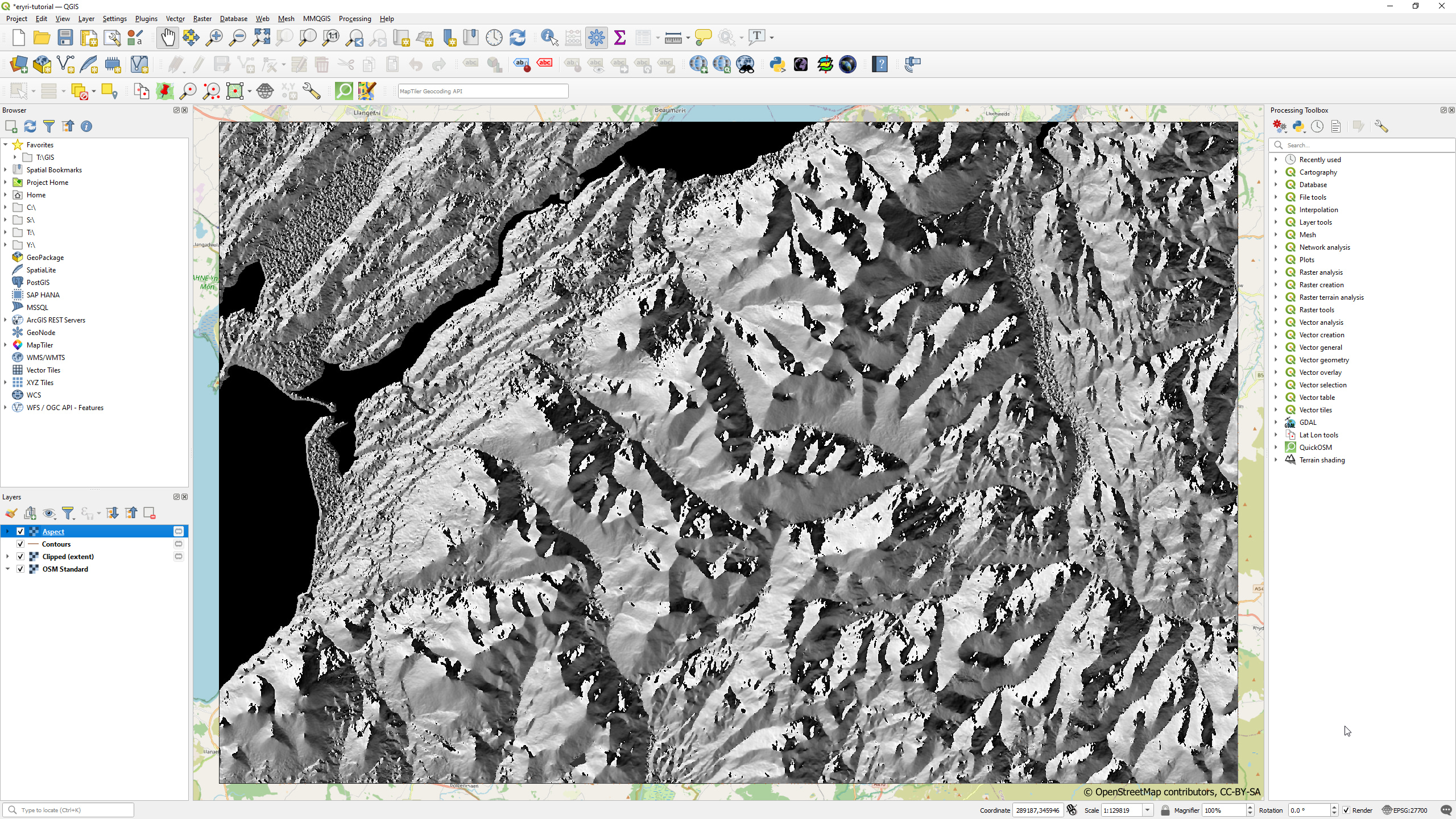
Aspect

• Select Raster → Analysis → Aspect... from the menu
• Set the input as the clipped elevation layer
• Click the Run button

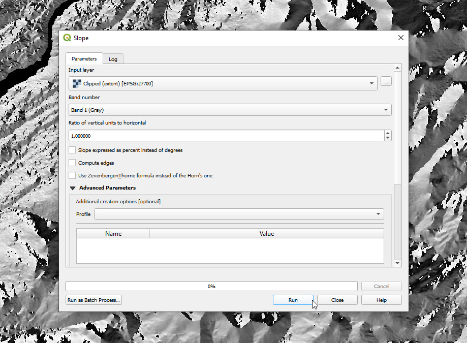
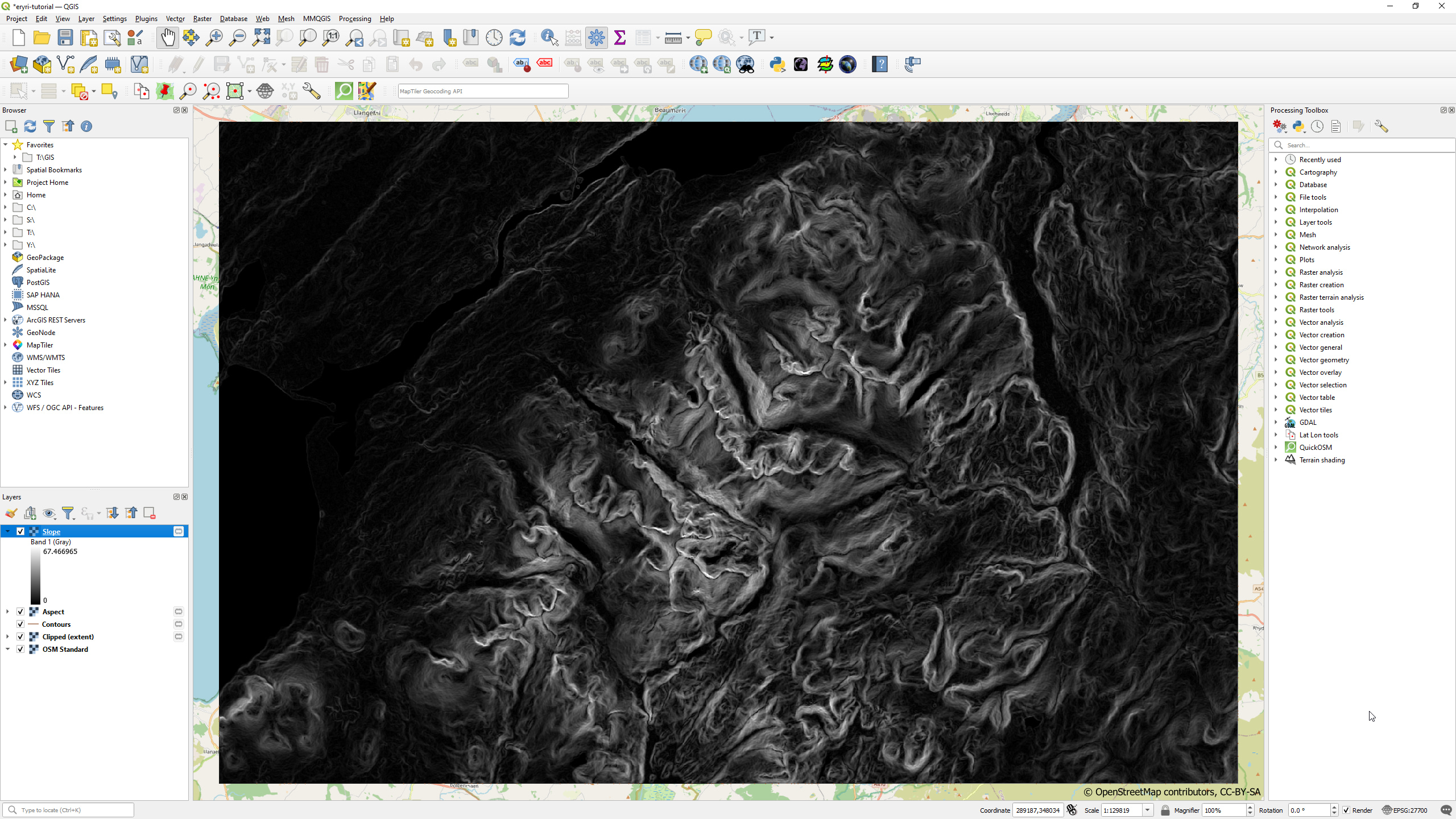
Slope

• Select Raster → Analysis → Slope... from the menu
• Set the input as the clipped elevation layer
• Click the Run button

You can play with the other settings if you like, though I’ve had good results leaving everything set to their default values.

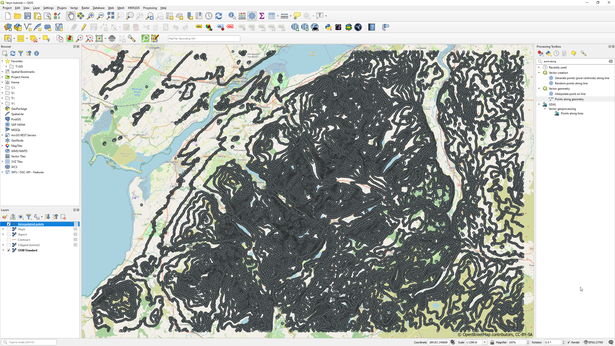
Place points along the contours

Our hachures will be drawn from various points along each contour line by sampling values from the aspect and slope rasters you generated. However, we can’t do that until we have the points along the contours, so let’s do that now.

You’ll need the Processing Toolbox open for this, so if you don’t already see it then you can open it via the Processing → Toolbox menu.

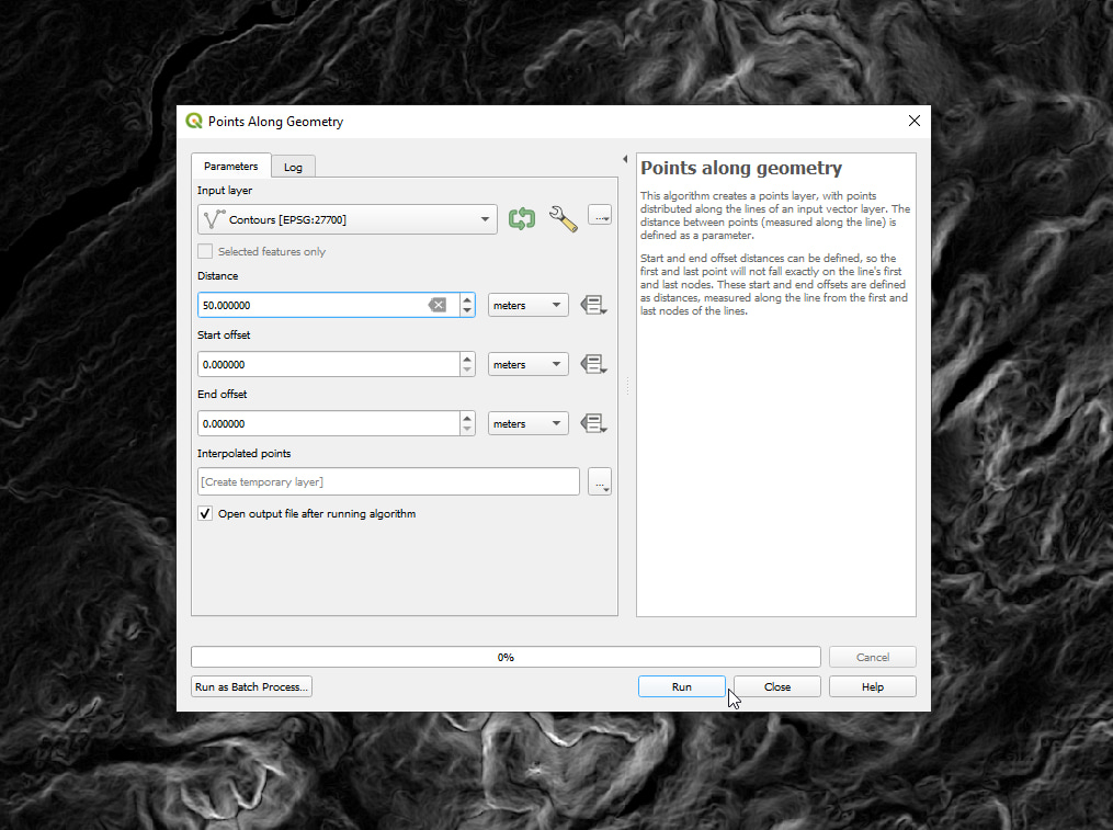
Now you can generate the points along the contours:

• Double-click Vector geometry → Points along geometry from within the toolbox, or type Points along geometry in the search bar
• Set the input as the contours layer
• Set the distance to something reasonable for your chosen location — this will be the interval between each hachure line (I used 50 metres)
• Click the Run button

Give it a little while and you’ll be presented with a lot of points on your map, each following one of the contour lines. If you inspect one of the points you’ll see that they contain some useful information for our hachures, namely an angle value relative to that point on the contour.

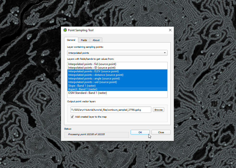
Sample the aspect and slope values

There is one more step before we can generate the hachures — sampling the aspect and slope values at each of the contour points. This is necessary as we’ll be using them to impact things such as the length, width and opacity of the hachure lines.

There are two ways to do this:

• Use Raster analysis → Sample raster values from the toolbox
• Use the Point Sampling Tool plugin

While both work, the toolbox approach requires multiple steps to sample both raster layers so we’ll be using the Point Sampling Tool for this tutorial.

• Install the Point Sampling Tool plugin if you haven’t already
• Ensure that the slope and aspect raster layers are visible in the layers panel
• Select Plugins → Analyses → Point Sampling Tool... from the menu
• Set the input to the contour points layer
• Select the contour points layers as well as the slope and aspect raster layers
• Set the output directory to the one you created at the beginning

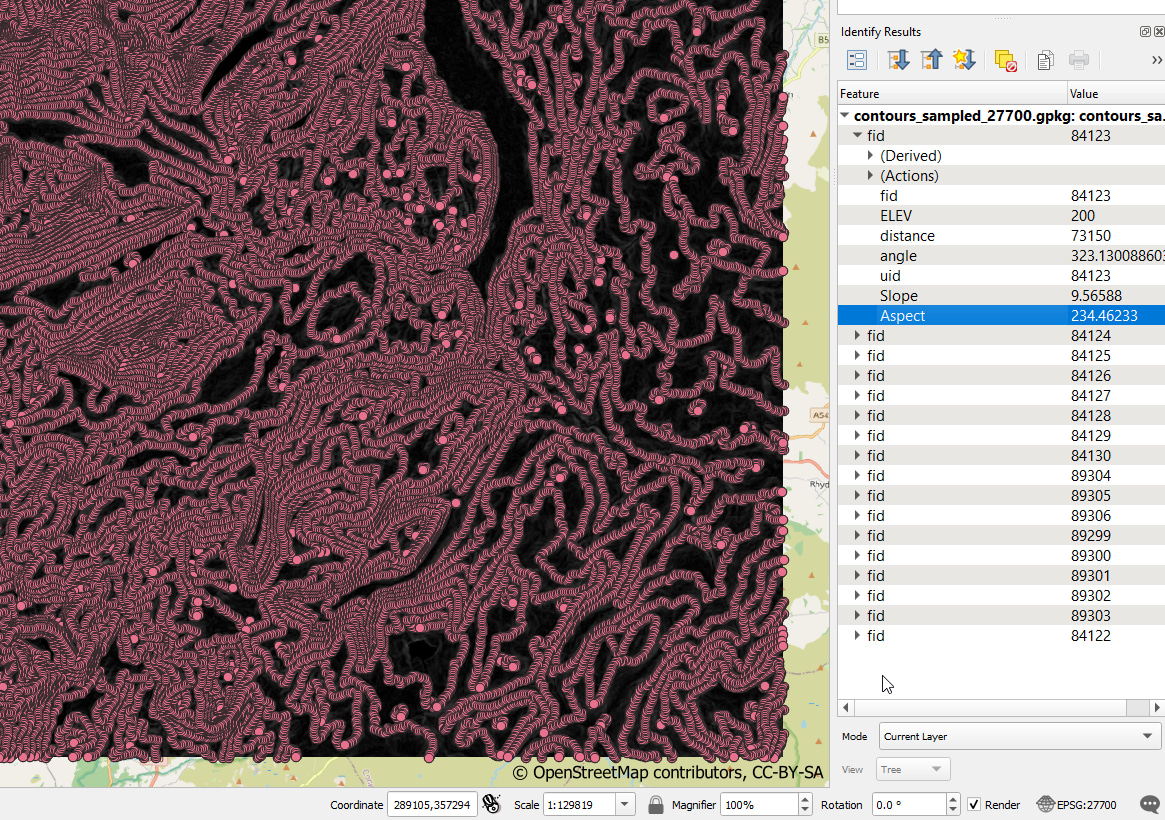
If you get an error about unique IDs then you may need to generate unique IDs for each contour point using the field calculator in QGIS. Sometimes I’ve had issues with the Point Sampling Tool and other times it’s worked without a problem.

---

Once the sampling is finished you’ll have a new point layer the contains the aspect and slope values at each contour point.

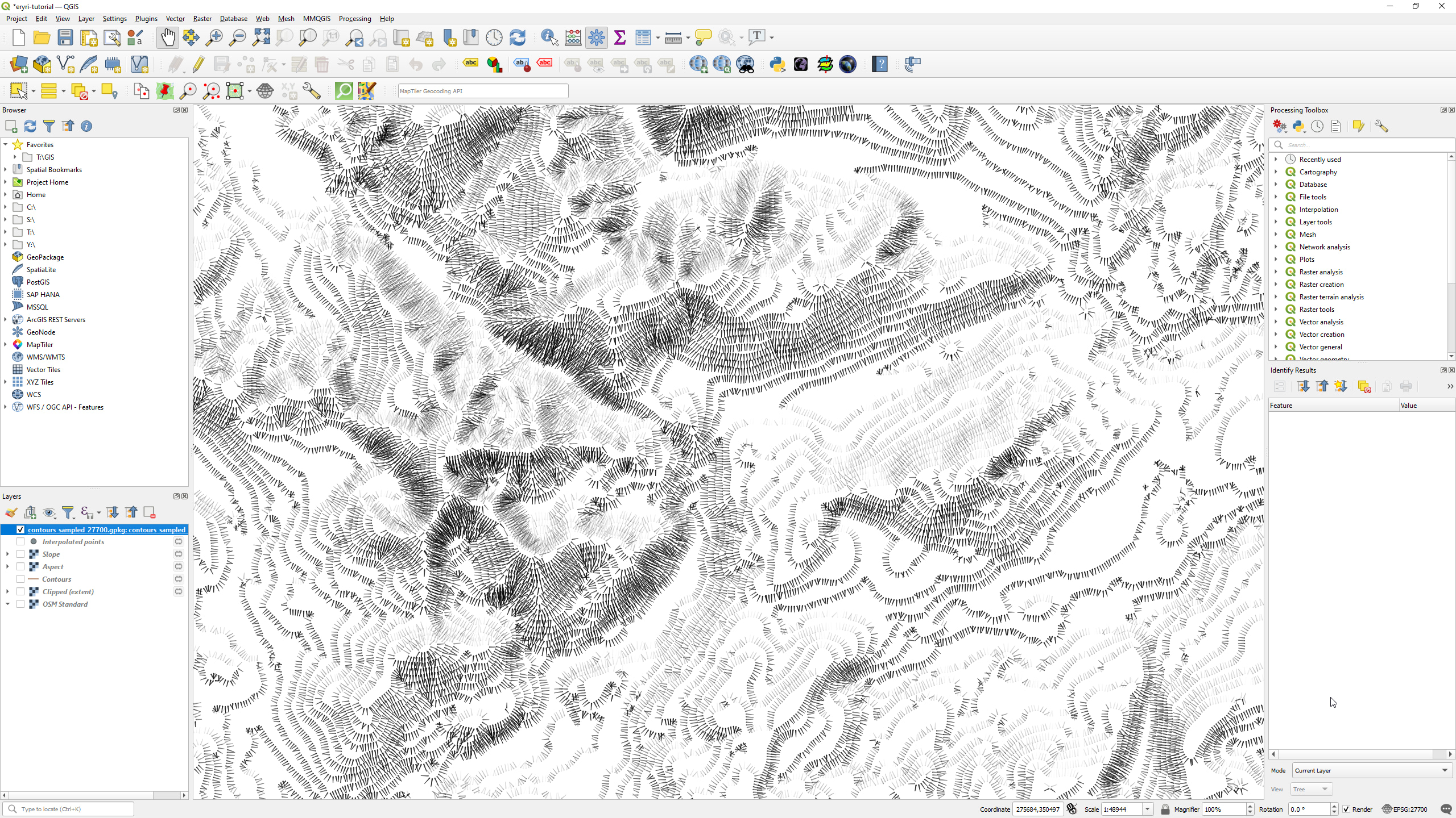
Basic hachure styling

Now the fun part can begin — styling the points to look like hachures! So first clean up the map by hiding all the layers aside from the sampled points layer, and then we can get cracking.

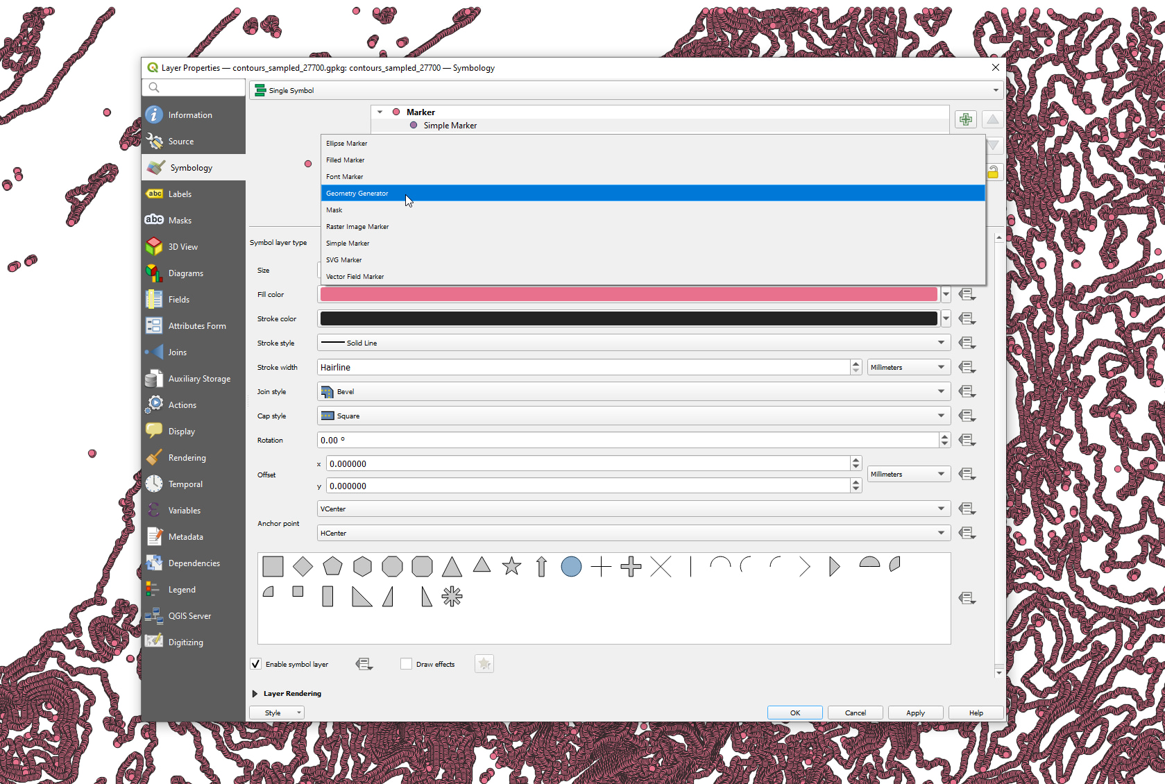
If you double-click on the sampled points layer then you’ll open up the layer properties panel. Select the Symbology tab if not already open by default — this is where we are going to live for the near future.

We need to turn the points into lines somehow, and there are countless ways to do this — some are particularly verbose. Fortunately QGIS has a feature called geometry generators, which can be used to (surprisingly) generate geometry using logic that you define. We’ll be using a geometry generator to create a line at each contour point using all the values that we just prepared.

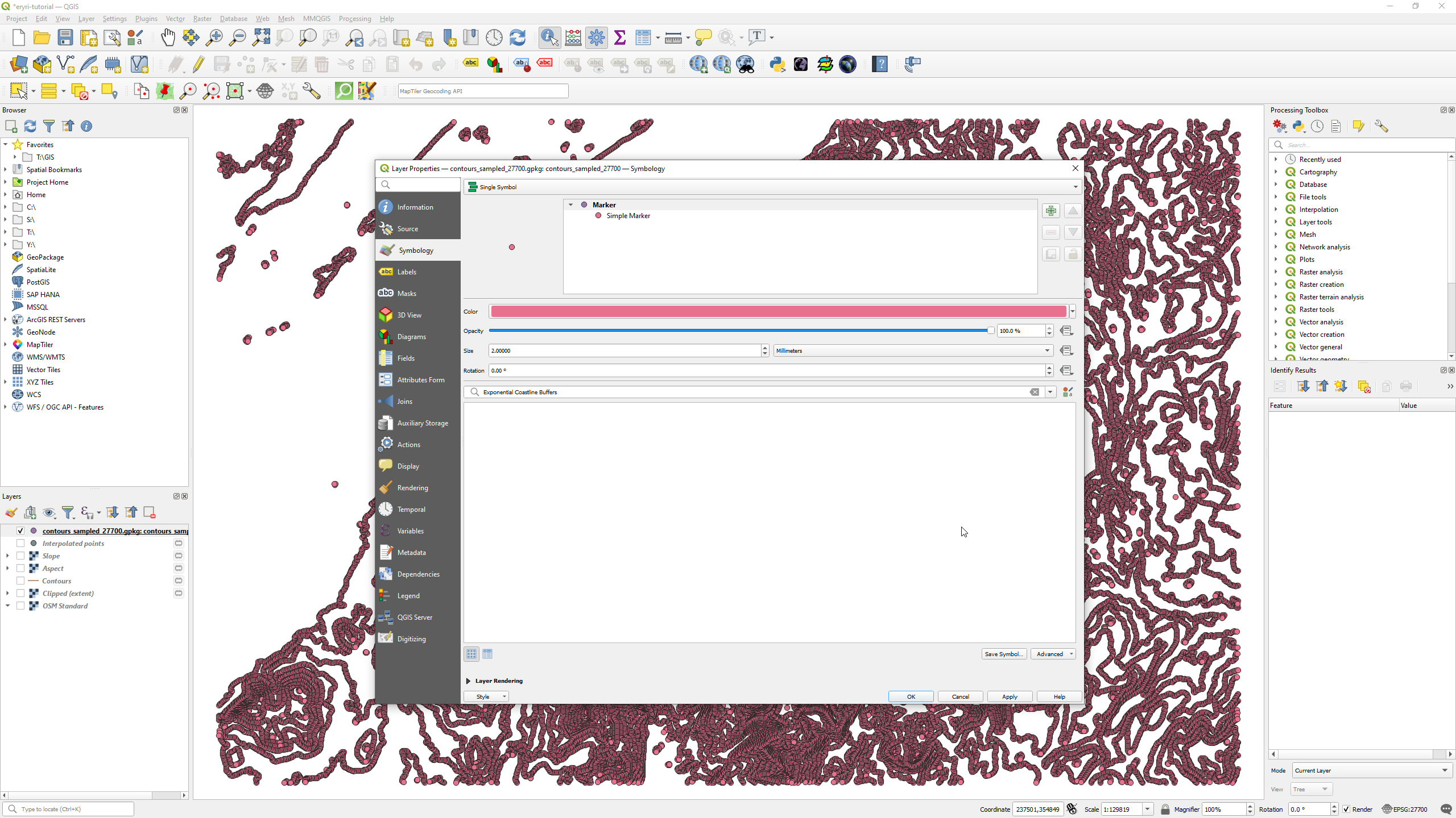
Click on Simple Marker in the symbology panel and change the layer type to Geometry Generator, which will display the geometry generator configuration. The default configuration is set to generate polygons — which we don’t want — so you’ll want to change the geometry type to LineString / MultiLineString.

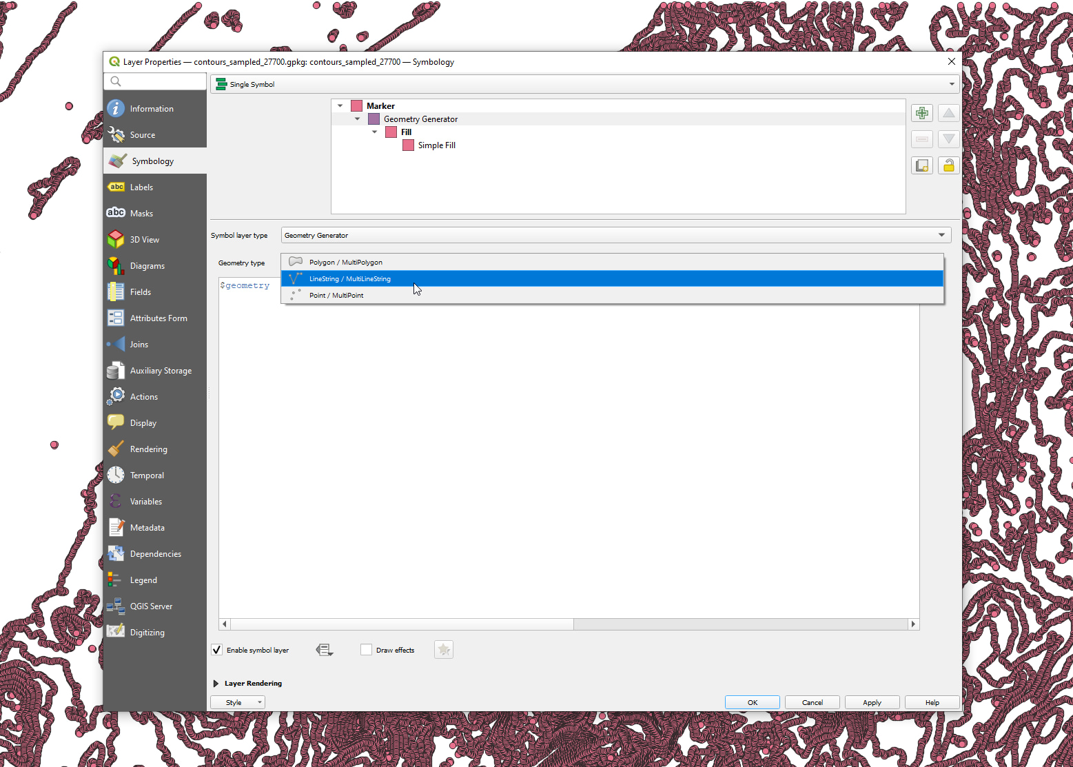
The text box that has $geometry in it is what is used to tell QGIS the geometry to put in place of the points on the map. The $geometry variable refers to the original geometry of the layer, so in our case it’s referring to each sampled point. We can use this in combination with the values we prepared to generate a line.

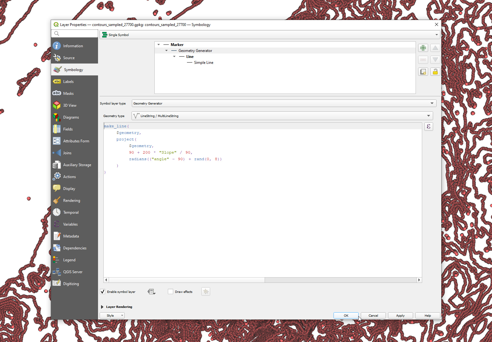
Replace $geometry with the following (which we’ll go through in a moment) and then click the Apply button:

make_line( $geometry, project( $geometry, 90 + 200 * “Slope” / 90, radians((“angle” - 90) + rand(0, 8)) ) )

Are those hachures?! Well kind of, though it’s a bit hard to see so let’s zoom in a bit…

Yup, those are looking mighty like *very basic *hachures! Though it’s not much use if this remains magic, so let’s break down what the geometry generator is doing.

Making a line using geometry generators

The first part is make_line(), which is a QGIS function that takes a point as input (our $geometry) and another point to draw a line to. We don’t have that other point yet so we need to calculate it based on the values we generated earlier.

Finding the end point of the hachure line involves the following general steps:

• Set the sampled contour point as the start point
• Find the bearing from the start point that’s perpendicular to the contour
• Find the distance from the start point to draw the hachure
• Project a point away from the start point using the bearing and distance

Fortunately QGIS has a helper function called project() that can do most of the work for us and avoid a bunch of trigonometry. It takes a start point, distance and bearing as inputs and the result is a new point at the given distance and bearing from the start point.

Finding the line bearing

Finding the bearing is relatively simple as we already have the angle of the sampled points along the line of the contour. We want the angle perpendicular to the contour so all you need to do is subtract 90 degrees and you get a bearing pointing away from the contour line.

We’ll also add a little bit of quirkiness to the lines by adding a random value between 0 and 8 degrees. Then all that’s left to do is convert the bearing into radians, as expected by the project() function.

radians((“angle” - 90) + rand(0, 8))

Finding the line distance

Finding the distance looks more complicated, though in reality there’s not a lot going on. We could also set the distance the same for each hachure line, though that would look very uniform and boring.

In our case we want to change the length of the hachure depending on the steepness at that point — longer for steeper, shorter for flatter. The slope values are an angle between 0 and 90, with 0 being flat ground and 90 being a vertical cliff. We can use this to find a dynamic distance value, though there’s a little math to apply first.

The first part is to convert the slope value to a range between 0 and 1, which we can then use to multiply into any range that we want. Given that we know the slope values are between 0 and 90 then you can divide the value by 90 to get a unit range between 0 and 1.

“Slope” / 90

From there we can multiply the unit range by whatever value we want. This part is up to you but given the values are in metres I found 200 metres a good range, plus an extra 90 metres so no line is shorter than that — the total range being between 90 and 290 metres.

90 + 200 * “Slope” / 90

Feel free to fiddle with the first two values as they will have a big impact on the hachure lengths depending on your map scale. You could even take things a step further and make this calculation independent of map scale, though that’s an exercise for another day.

Shading hachures using sun direction

Things look half-decent already, though we can do better. We can start by changing the opacity of the hachure lines depending on their angle, similar to hill-shading.

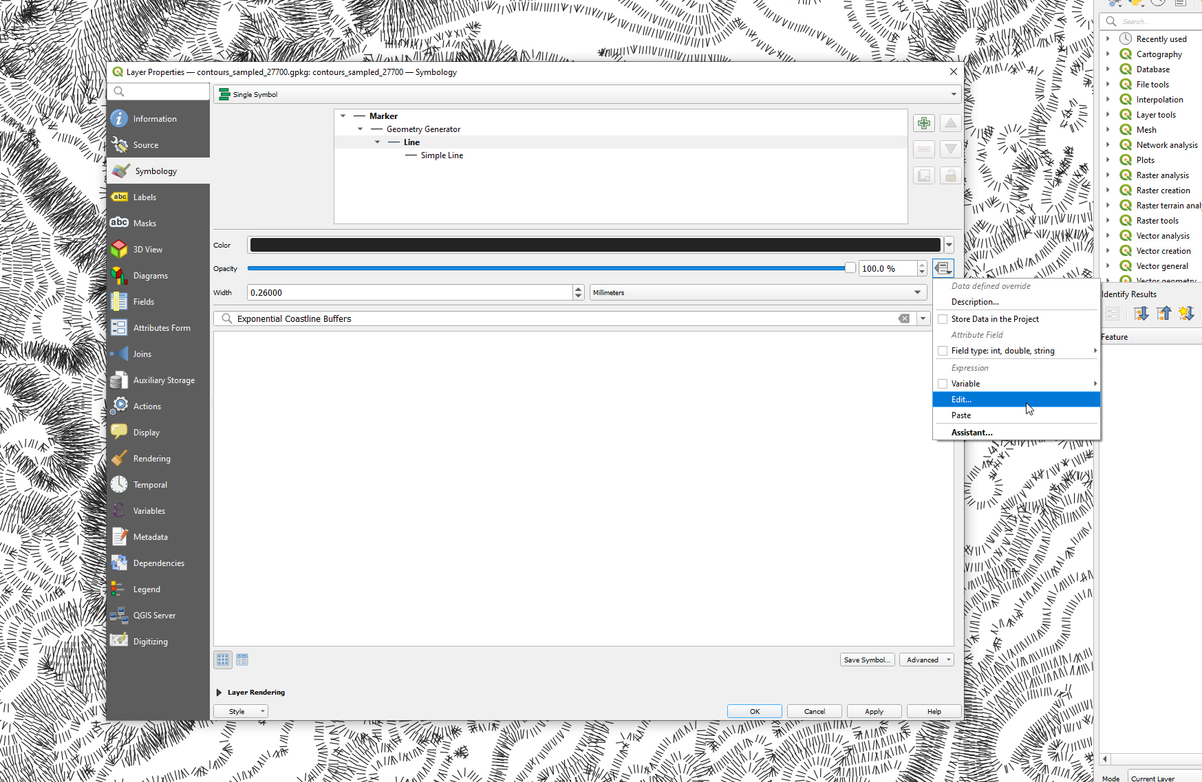
We already have everything we need to do this so go back into the geometry generator symbol and click on the Line symbol within it. We want to dynamically change the opacity so click on the button to the right of the opacity slider and click on Edit....

This will open the expression editor and the result of whatever you enter here will be set as the opacity, which expects a value between 0 and 100. In our case we want anything facing north to be transparent, and shifting to black when facing south. We can use the aspect value for this, which is an angle between 0 and 360 degrees clockwise from north.

There are a few more things we need to do:

• Subtract 180 from the aspect value to get a value between -180 and 180 degrees (with 0 being south)
• Convert that into an absolute value so the result is always between 0 and 180 regardless of whether you go clockwise or anti-clockwise
• Divide the result by 180 to get a unit range with 0 being south and 1 being north
• Subtract the result from 1 to flip the range so 0 is north and 1 is south
• Multiply the result by 100 to get a range between 0 and 100

All together you get the following expression:

100 * (1 - abs(“Aspect” - 180) / 180 )

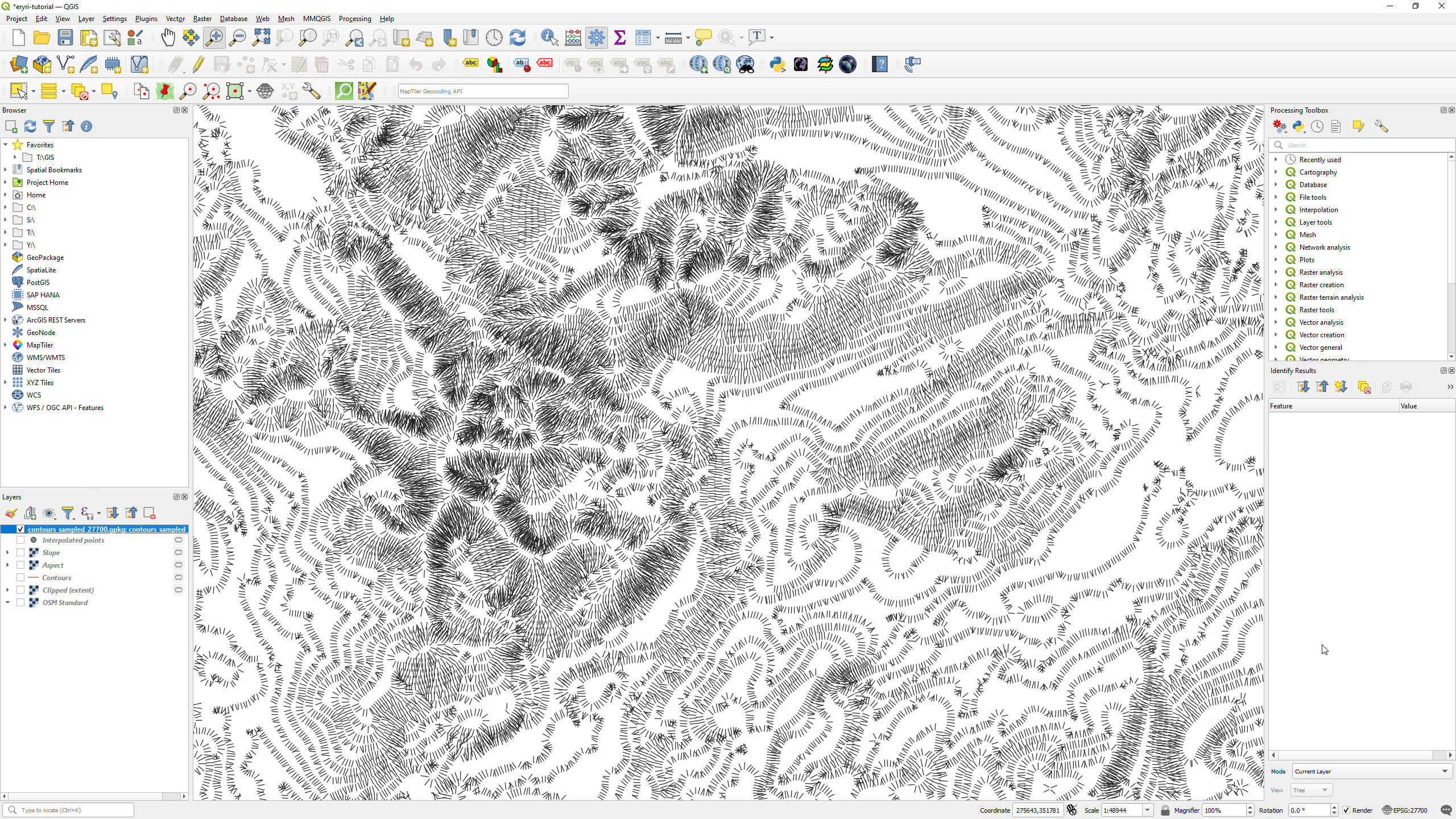
Plug this in, click the OK button and then click the Apply button to see the results on the map.

You will probably want to experiment with this expression so that 0 is at the northwest, though I’ll leave that as a follow-up exercise.

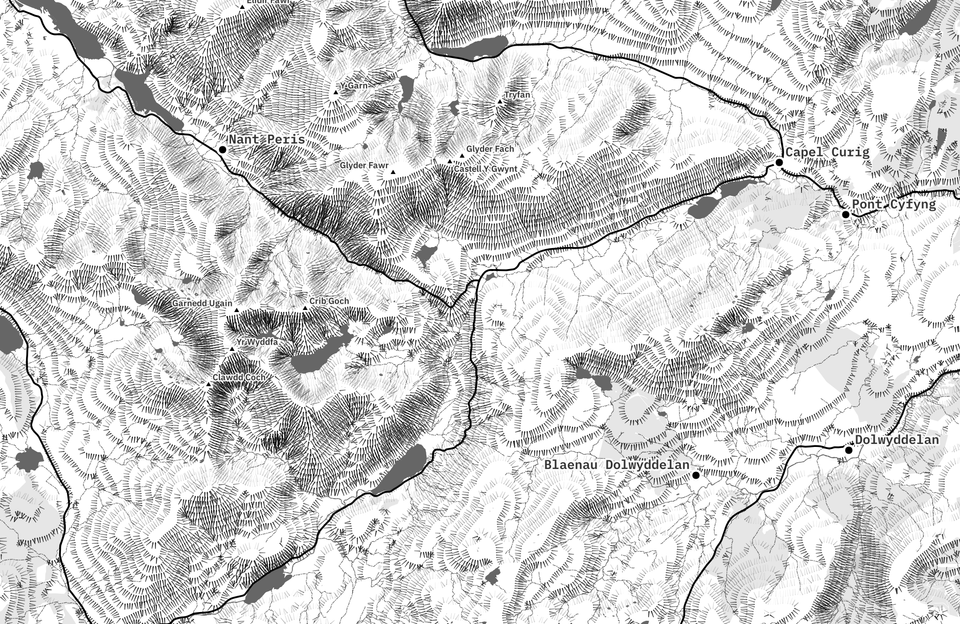
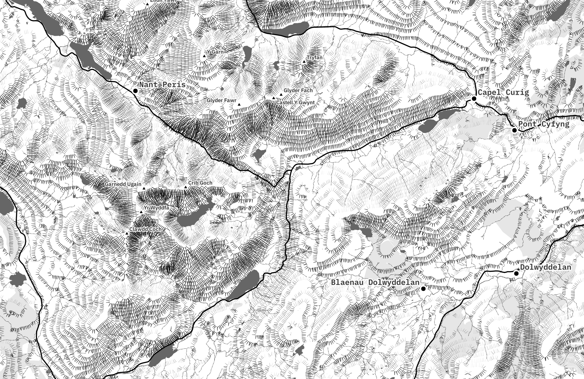
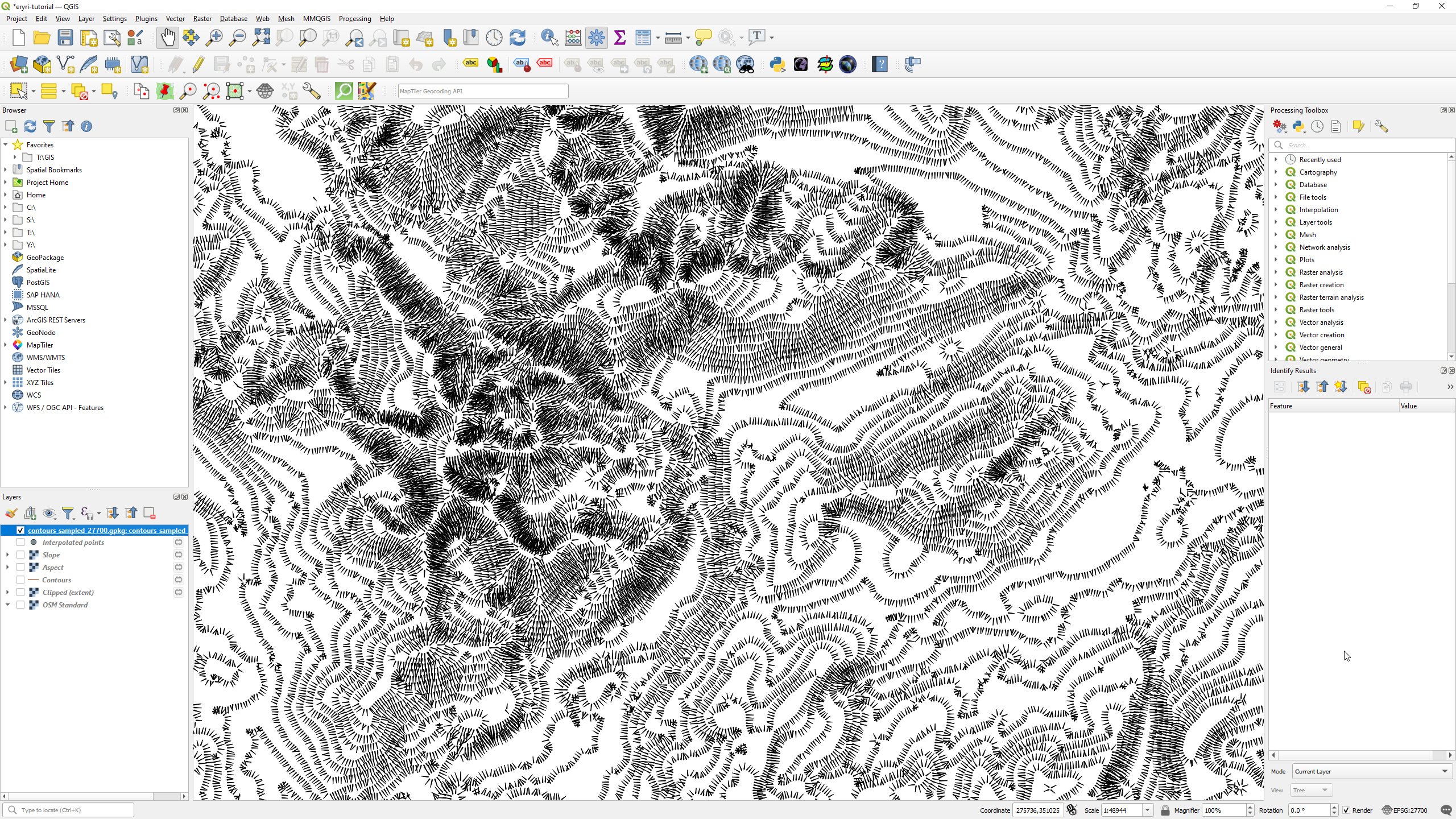
Tapered hachures

We can take things a step further and taper the hachures so they are slightly thicker at the base of the contour, tapering to a point as they move away from the contour.

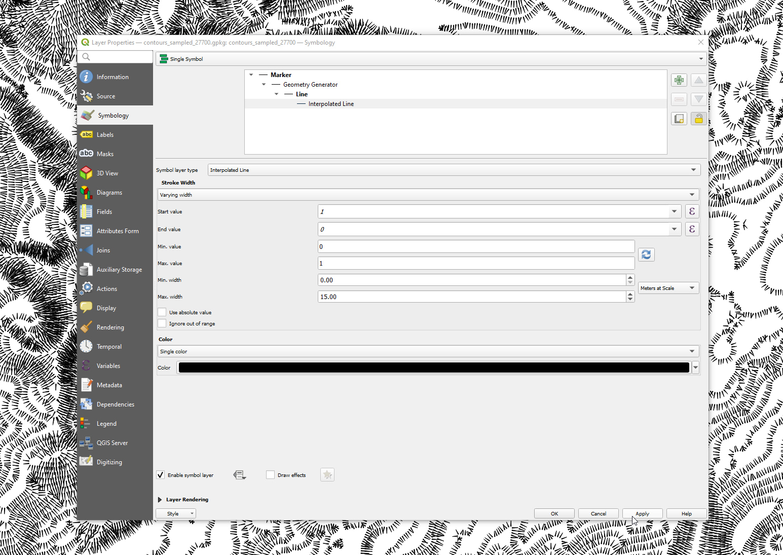
Open up the symbology panel again and select the Simple Line within the geometry generator for the hachure layer. We’re going to use a new feature in QGIS 3.20 called interpolated lines, so select that from the layer type dropdown.

We want the lines to be thicker at one end so select Varying width from the stroke width dropdown. You’ll then be presented with a bunch of options, though we’re only interested in a couple of them.

Specifically, set the following values:

• Set the start value to 1 so the base is the thickest (this isn’t the width)
• Set the end value to 0 so the tip is the thinnest
• Set the min value to 0
• Set the max value to 1
• Set the min width to 0 so the tip tapers to nothing
• Set the max width to 15
• Change the units from Millimeters to Meters at Scale

If you save and apply this you’ll see an ever-so-slight tapering of the hachure lines — they may also look a bit thicker. You can play with the min and max width values to tweak the style, though you shouldn’t need to change any of the other values.

You’ll also notice that the opacity has stopped working, so let’s fix that.

Opacity with tapered hachures

A quirk I’ve noticed with the interpolated lines feature is that it completely ignores the opacity set further up the chain in the layer symbology. This results in the tapered lines ignoring the dynamic opacity that we previously set.

The simplest workaround for this is to set the opacity within the interpolated lines themselves. So open up the symbology panel again and select the Interpolated Line from before.

We have to jump through one more hoop to set the opacity as you can’t set it on the interpolated line when its colour mode is set to Single color, so open up the colour mode drop-down and select Varying color.

Use the following settings:

• Set start and end values to 1 - abs("Aspect" - 180) / 180
• Leave interpolation as linear
• Double-click the colour for 0 and set it to transparent black
• Double-click the colour for 1 and set it to 75% black

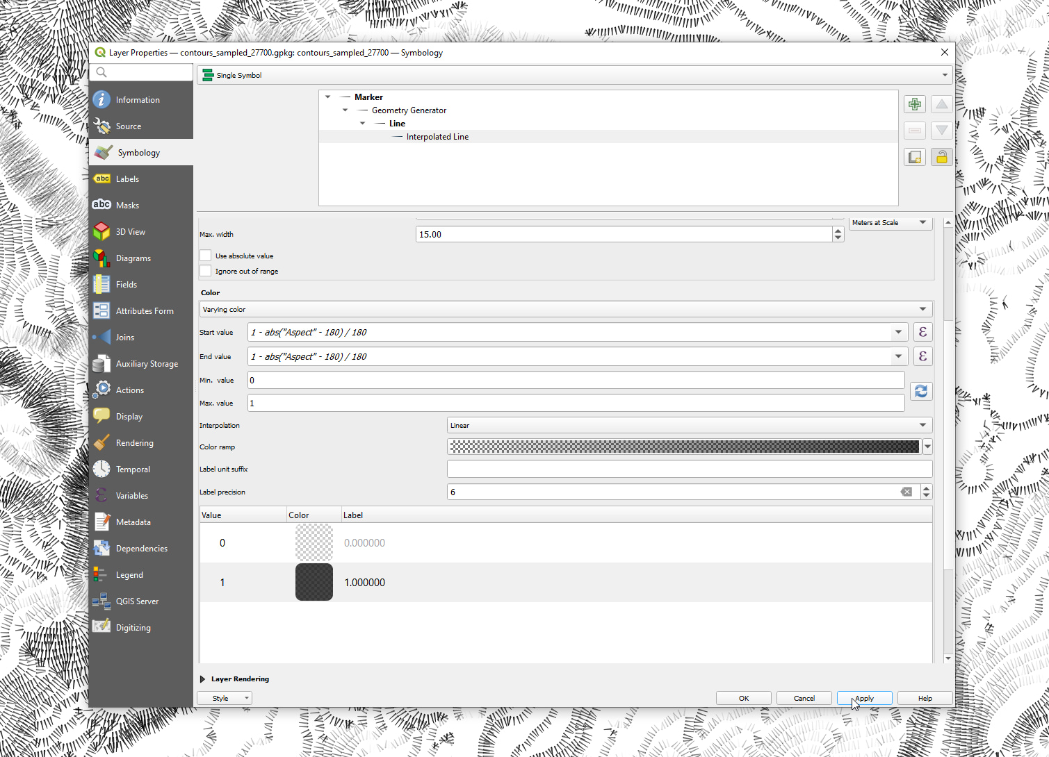
Click the Apply button and the hachures should be tapered and change opacity depending on the angle from the north.

---

There seems to be a bug with the interpolated line feature that resets the varying colour start and end values when you next open the symbology panel.

If you notice your tapered lines losing the opacity then check that the start and end values are still set to 1 - abs("Aspect" - 180) / 180 before checking anything else.

---

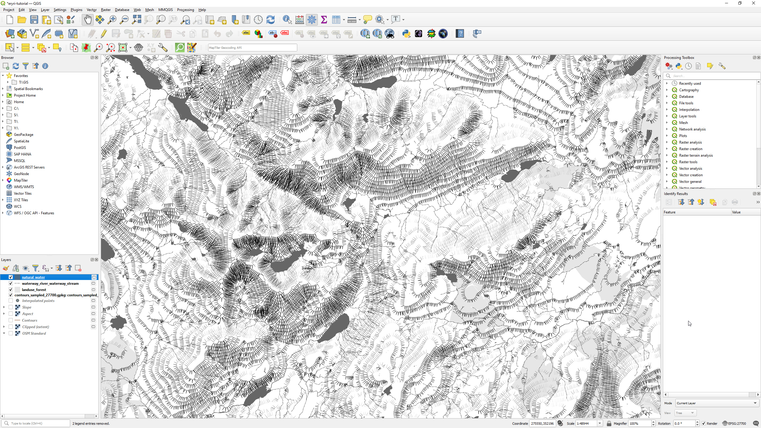
Adding context to the map

We’re technically done with the hachures at this point, though the map is looking a little bare. Let’s add some features from OpenStreetMap to provide a bit of context and make things look even nicer.

We’ll use the QuickOSM plugin to save time with gathering data from OpenStreetMap, so go ahead and install that if you don’t have it already.

It’s possible to download all the OpenStreetMap features we need as one big request, though this will result in them all being contained in the same layers and requiring some advanced styling to filter and separate them. In this tutorial we’ll be requesting independent features as separate requests to keep things simple.

Planting the trees

One of the simplest ways to add a bit of detail to the map is to highlight areas that contain forests and trees. We can do this using the landuse=forest tag on OpenStreetMap.

Open up the QuickOSM plugin by clicking the button on the toolbar and then use the following settings:

• Set the key to landuse
• Set the value to forest
• Select Layer extent from the drop-down underneath the key/values
• Select the sampled contour points as the extent layer

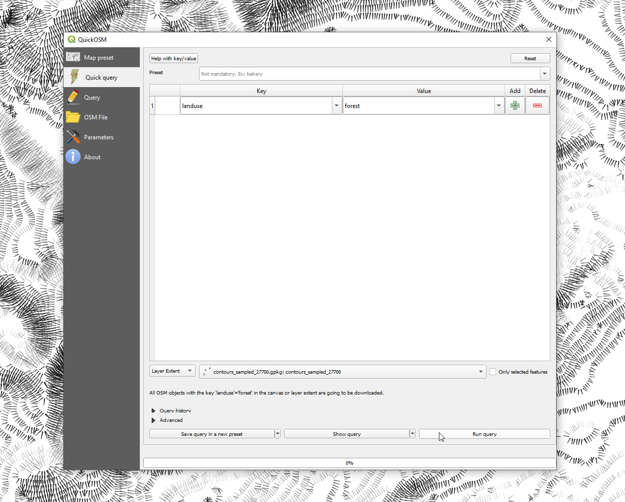
Click the Run query button when you’re done and wait for the data to download from the Overpass API. If everything worked then you’ll see a bunch of polygons on the map.

You can immediately hide or remove the line and point layers as we won’t be using that data for the forests. Then double-click the forest polygons layer and open the symbology panel.

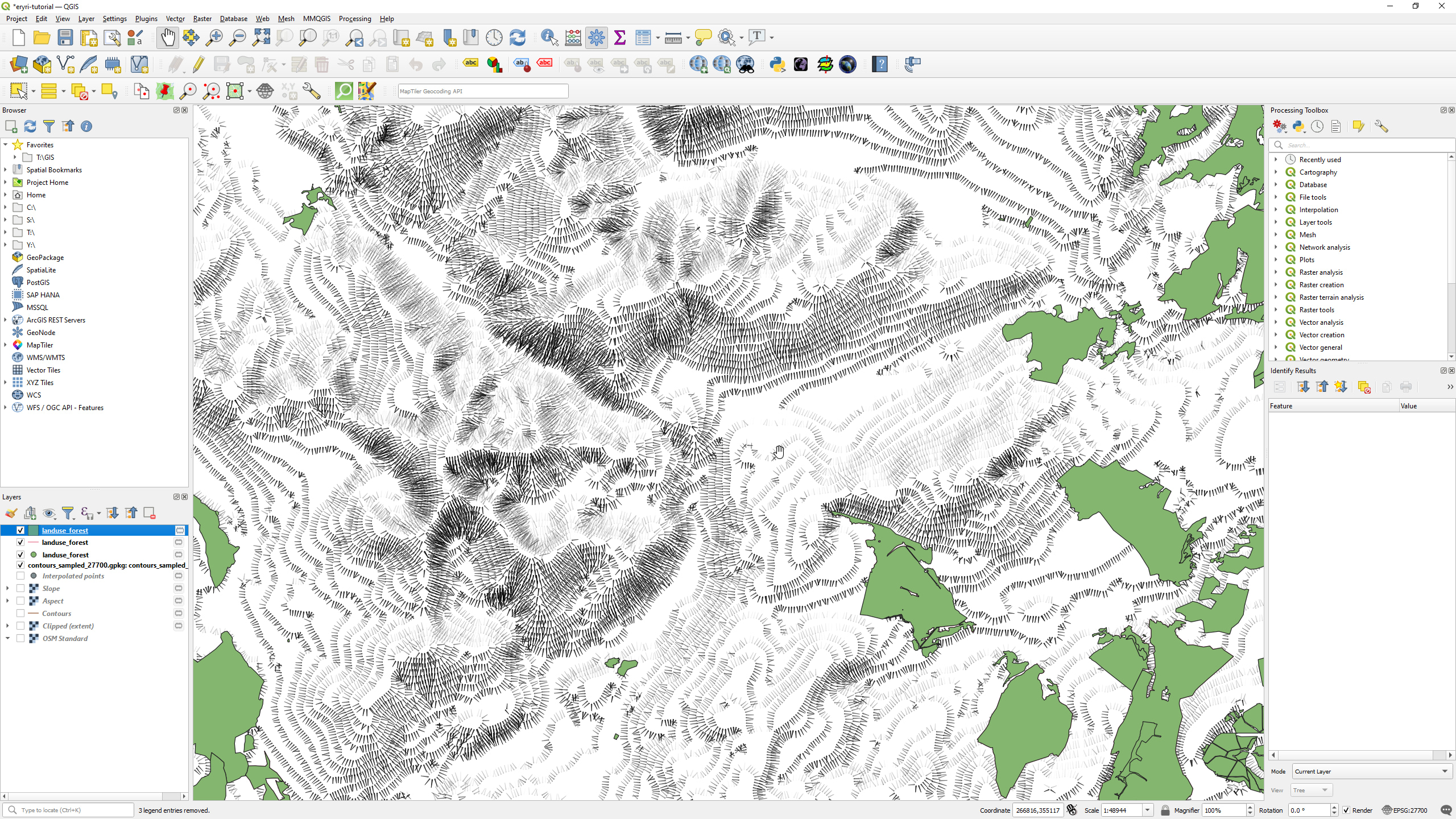
Set the forest styling to whatever you prefer, though if you want to match the style of the tutorial then set the opacity to 10% and set the fill colour to black. Also, set the stroke style to No Pen in the Simple Fill settings.

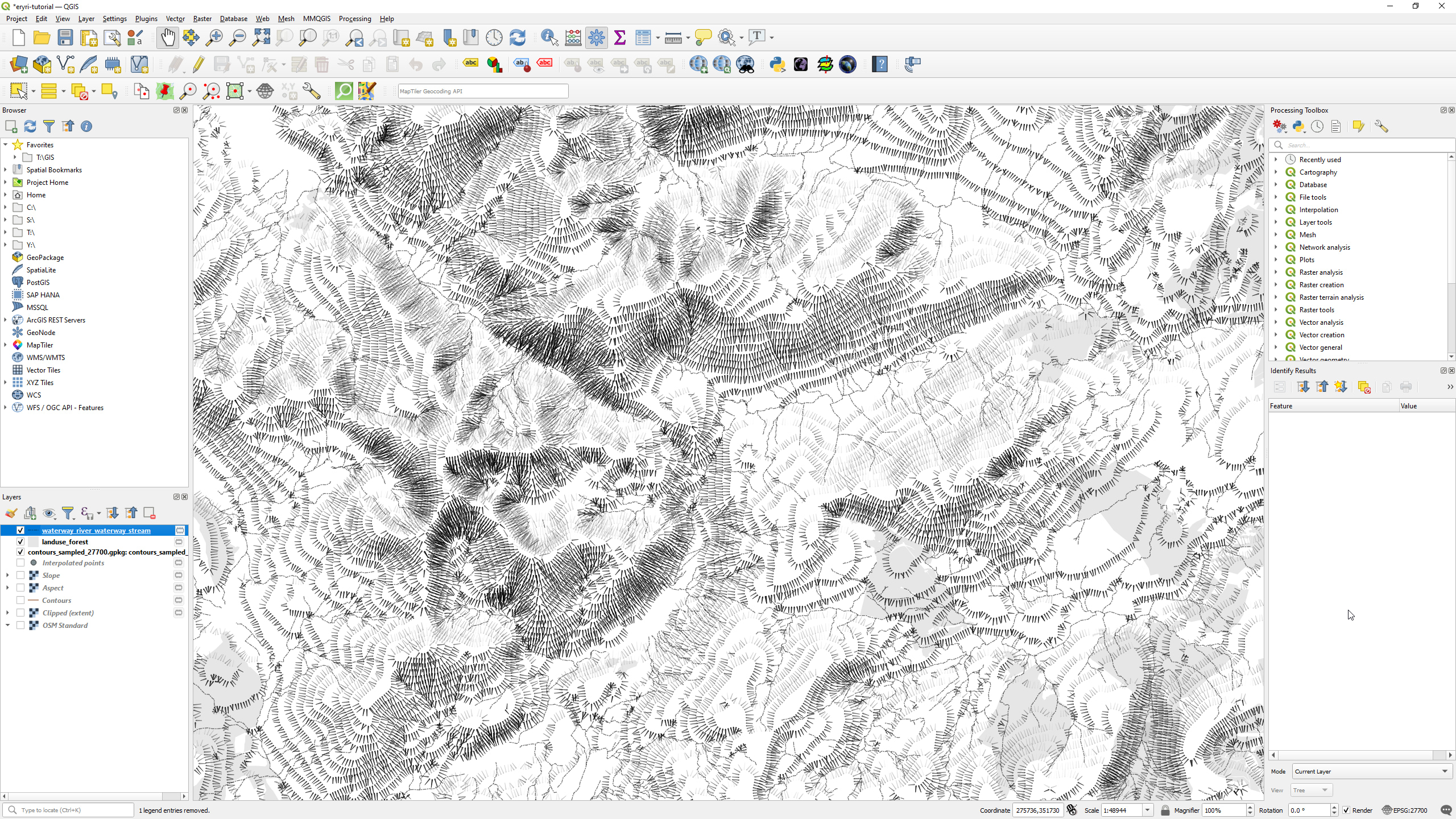
Carving the rivers

Next we’ll add the rivers and streams, which will provide a huge amount of detail for mountainous areas like Eryri.

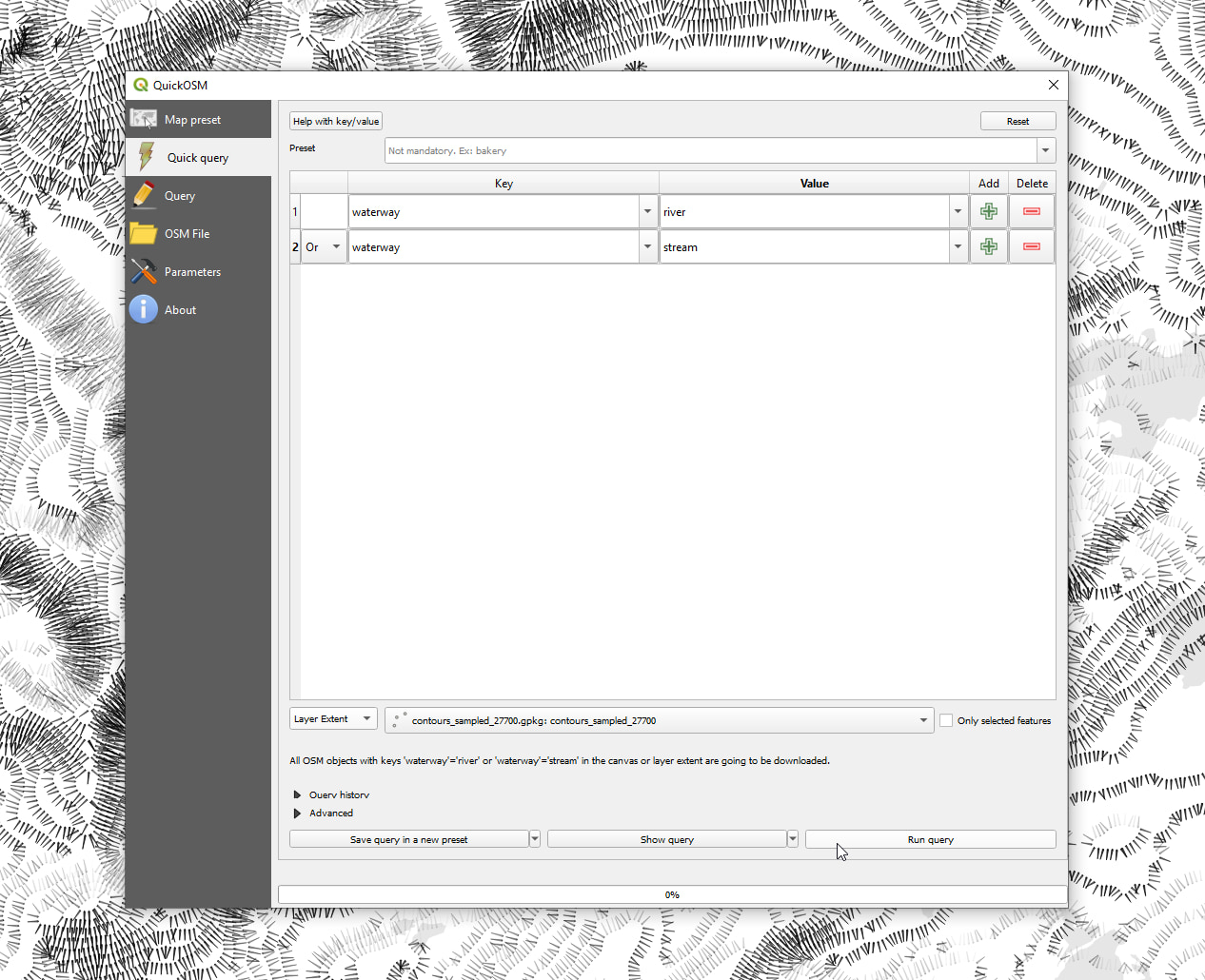
Open up QuickOSM as before and use the following settings:

• Set the key to waterway and the value to river
• Click the green plus button to add a new row
• Set the comparison on the new row to Or
• Set the second key to waterway and the value to stream
• Set the extent and layer as before

Run the query and you’ll see a bunch of lines appear on the map, and potentially some points. We don’t need the points so hide or remove that layer, then open up the symbology panel for the waterway lines layer.

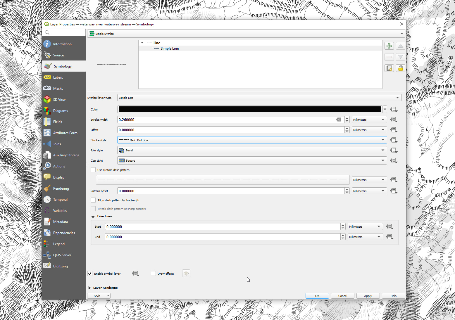
Select the Line symbol and use the following settings (or your own):

• Set the colour to black
• Set the opacity to 60%
• Select the Simple Line symbol and change the stroke style to Dash Dot Line

Filling the lakes

River and streams are great, though they are incomplete without the lakes that they feed in and out of. Open up QuickOSM again.

• Set the key to natural and the value to water
• Set the extent and layer as before

We don’t need the lines or points so hide or remove those layers, then open up the symbology panel for the water polygons.

Set the water styling to whatever you prefer, though if you want to match the style of the tutorial then set the fill colour to 60% black — rgb( 102, 102, 102 ). Also, set the stroke style to No Pen in the Simple Fill settings.

Laying the roads

Next up roads, following the same process as before using the QuickOSM plugin.

• Set the key to highway and the value to primary
• Click the green plus button to add a new row
• Set the comparison on the new row to Or
• Set the key to highway and the value to trunk
• Set the extent and layer as before

We don’t need the points so hide or remove that layer, then open up the symbology panel for the road lines.

Select the Line symbol and use the following settings (or your own):

• Set the colour to black
• Set the width to 0.75

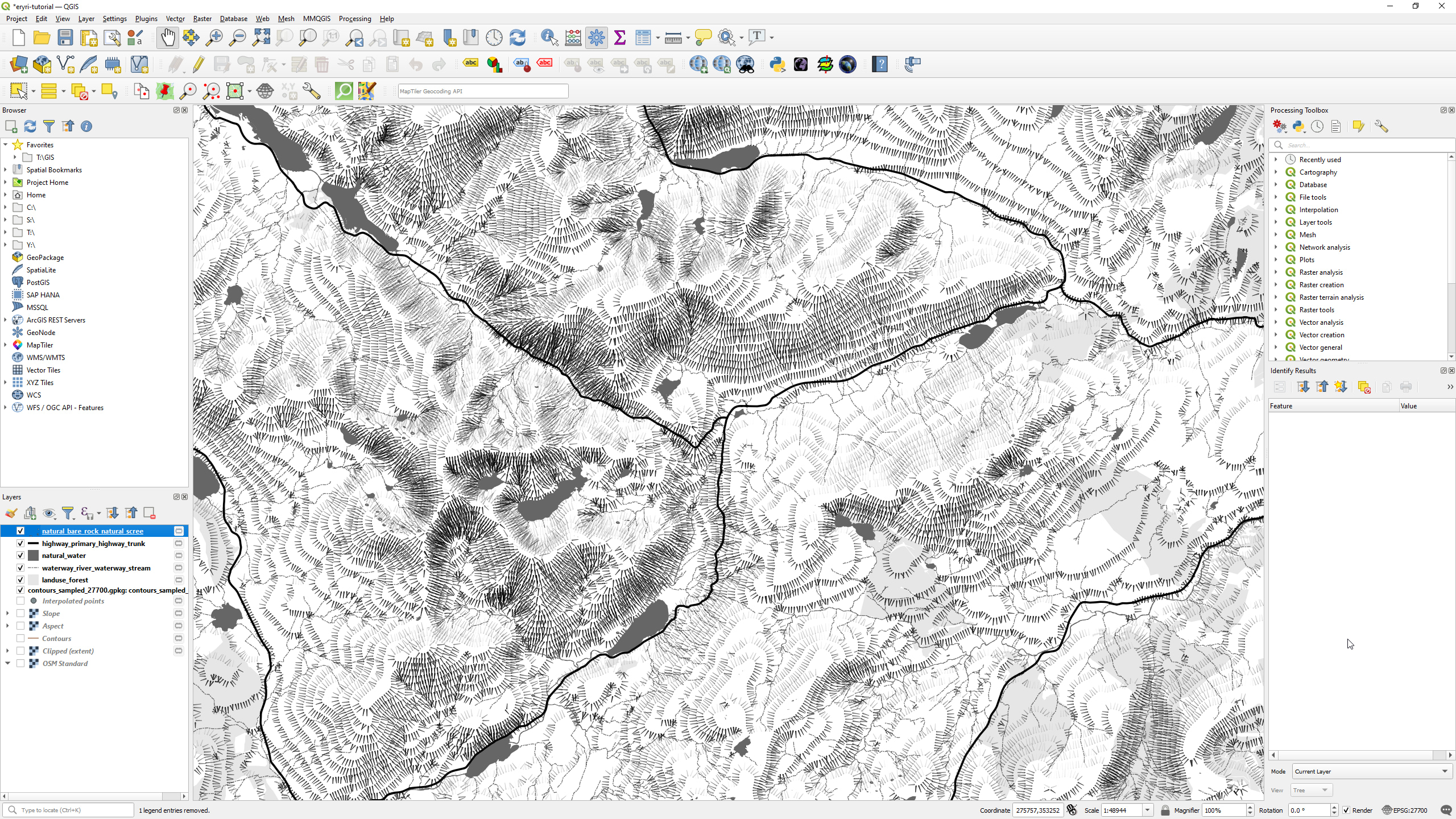
Sprinkling the rocks and scree

One extra bit of detail is to throw down some rocks and scree, especially if you’re following the tutorial in a mountainous location. Open up QuickOSM again.

• Set the key to natural and the value to bare_rock
• Click the green plus button to add a new row
• Set the comparison on the new row to Or
• Set the key to natural and the value to scree
• Set the extent and layer as before

We don’t need the points so hide or remove that layer, then open up the symbology panel for the rock polygons.

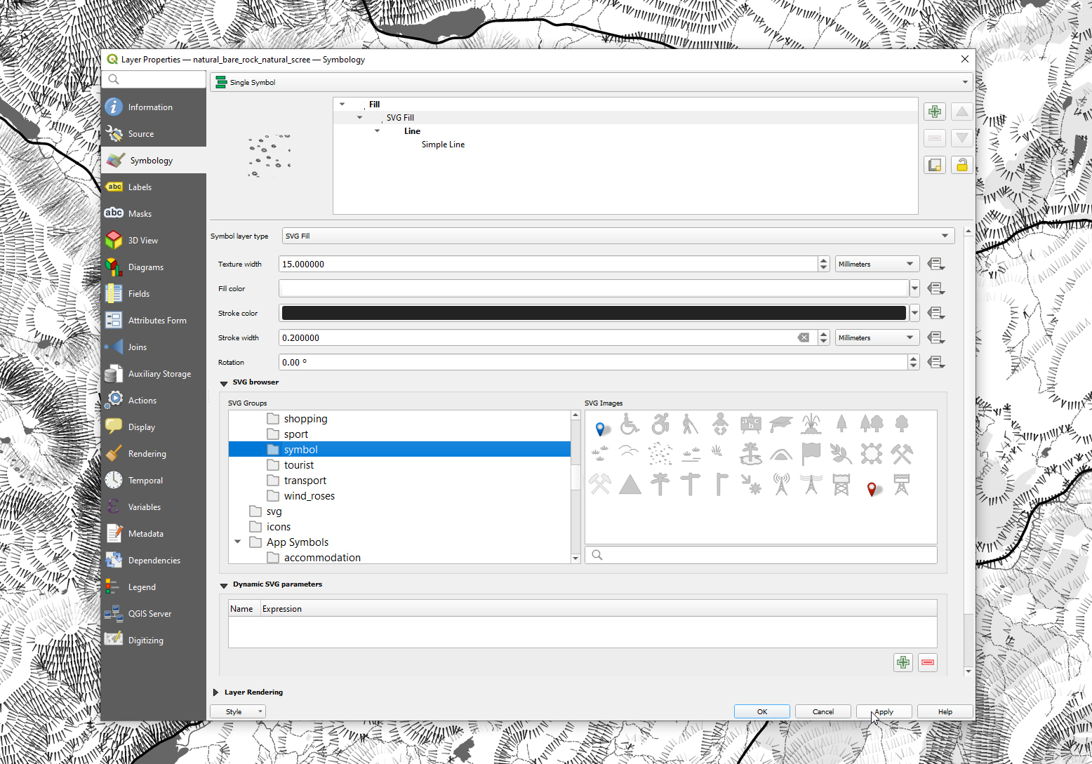
We’re going to add a rock pattern here so select the Simple Fill and then select SVG Fill from the layer type drop-down.

• Scroll to the SVG browser and click on the svg → symbol directory
• Select the quarry pattern (that looks like a bunch of dots)
• Set the texture width to 15, or whatever you prefer
• Set the fill colour to white
• Set the stroke style to No Pen in the Simple Line settings

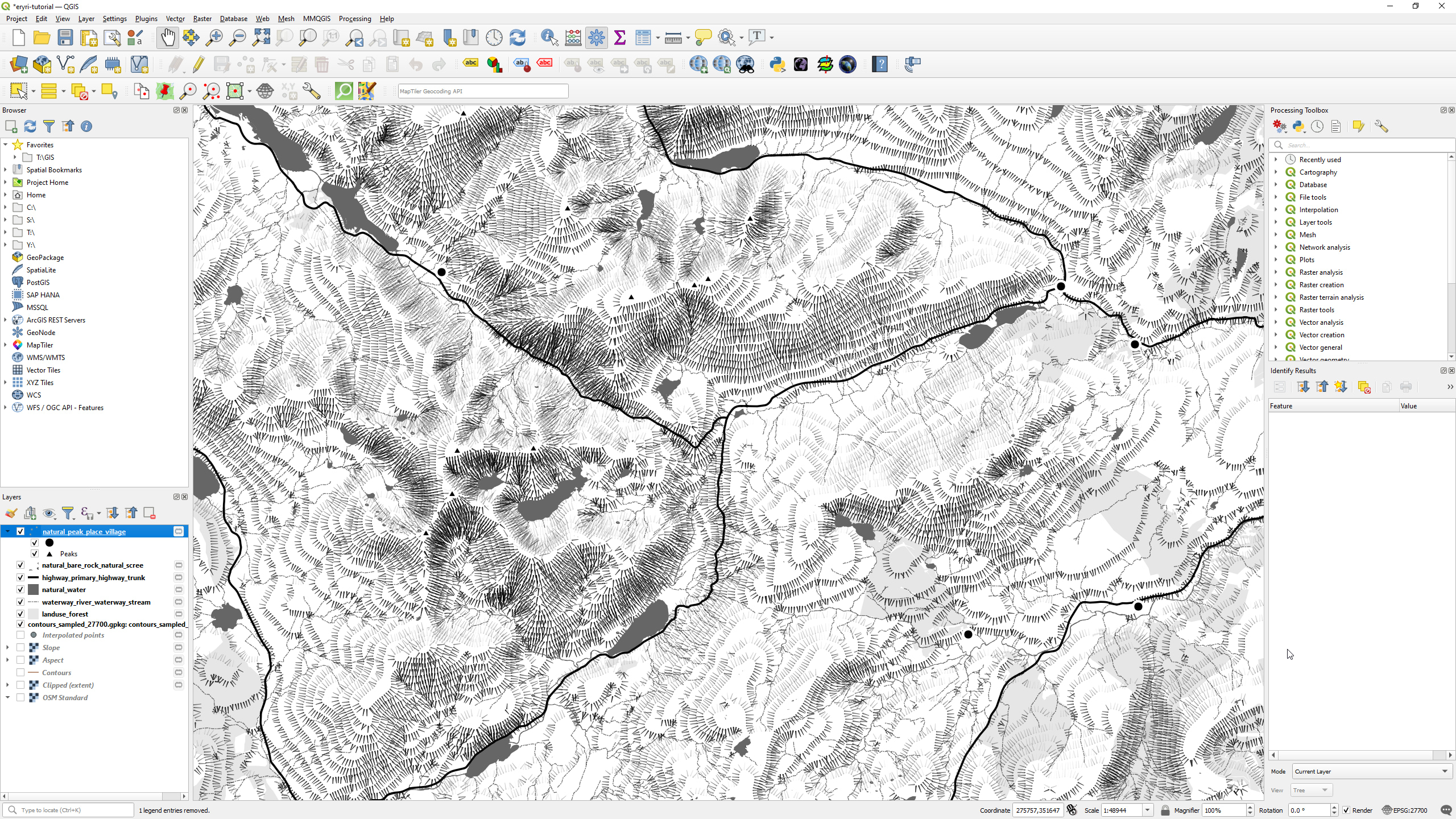
Labelling peaks and places

Finally it’s time to add some labels for nearby peaks and places in the area, so open up QuickOSM one last time.

• Set the key to natural and the value to peak
• Click the green plus button to add a new row
• Set the comparison on the new row to Or
• Set the key to place and the value to village (or whatever you prefer)
• Set the extent and layer as before

We don’t need the polygons so hide or remove that layer, then open up the symbology panel for the place points.

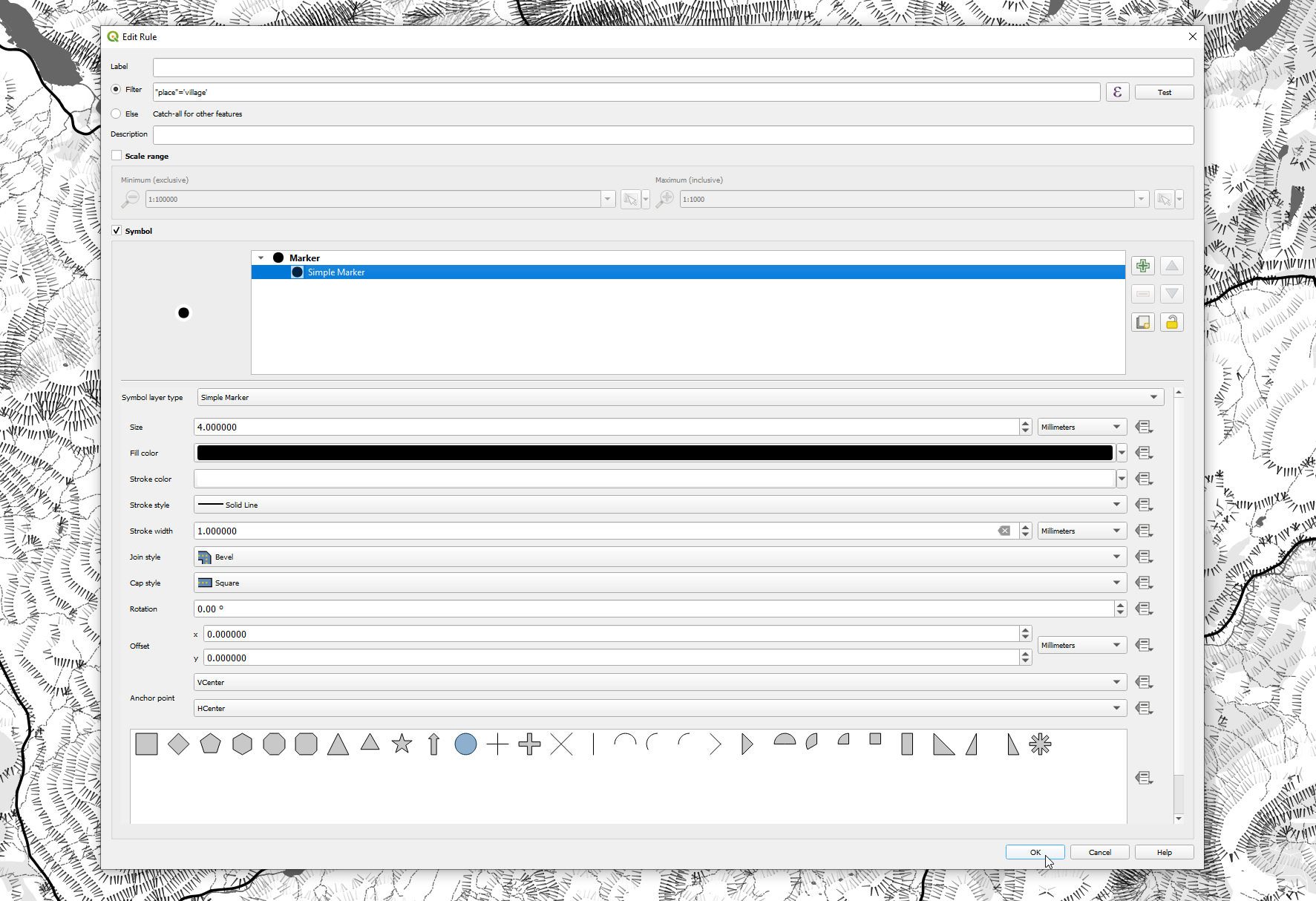
Villages and peaks are going to be styled differently so we’ll want to use a different method for setting up the styling this time. Change the symbology from Single Symbol to Rule-based.

Double-click the existing rule and use the following settings:

• Set the label to “Villages” (this is purely for your reference)
• Set the filter to "place"='village'
• Click on the Simple Marker
• Set the fill colour to black
• Set the stroke colour to white
• Set the size to 4
• Set the stroke width to 1

Let’s do the same for peaks, starting by clicking the green plus button at the bottom to add a new rule and then using the following settings:

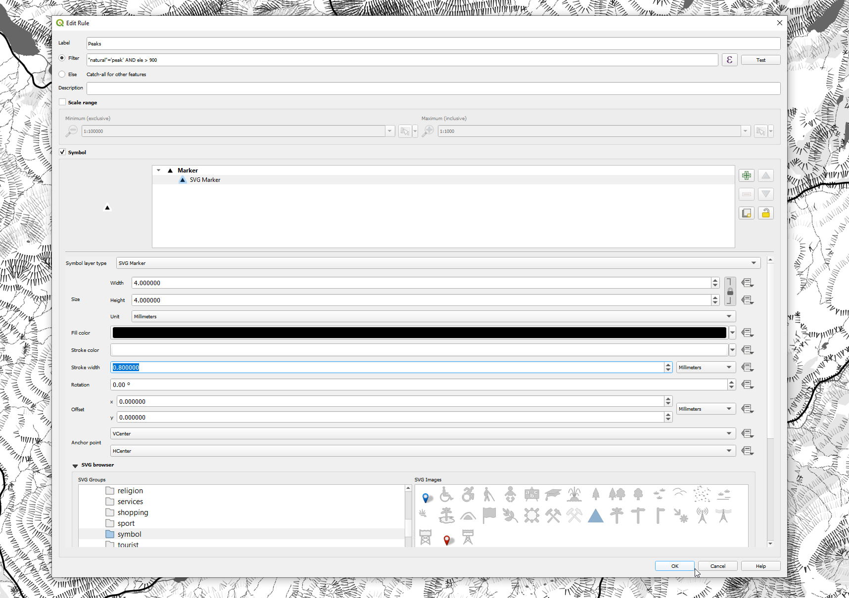
• Set the label to “Peaks” (this is purely for your reference)
• Set the filter to "natural"='peak' AND "ele" > 900 (only peaks over 900 metres)
• Click on the Simple Marker and set the layer type to SVG Marker
• Scroll to the SVG browser and click on the svg → symbol directory
• Select the peak symbol (that looks like a triangle)
• Set the fill colour to black
• Set the stroke colour to white
• Set the size to 4
• Set the stroke width to 0.8

If you click apply and close the symbology panel you can see the current progress — a bunch of dots and triangles where villages and tall peaks are located. This is good, though it’d be better if we knew what they were called.

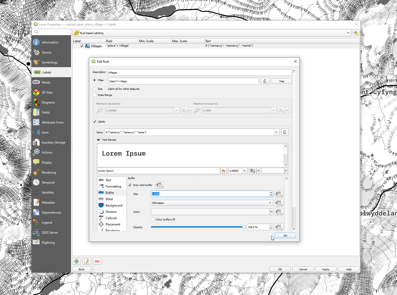
Open up the symbology panel again, select the Labels tab and then change No Labels to Rule-based Labeling. Click on the green plus button to add the first rule, and follow a similar process to the layer styling.

• Set the description to “Villages”
• Set the filter to "place"='village'
• Set the value to if ("name:cy", "name:cy", "name") (tries to use Welsh names)
• Click on Text and set the font to something fun (I’m using IBM Plex Mono)
• Set the text size to 15
• Click on Buffer and enable Draw text buffer
• Set the buffer size to 1.5
• Set the buffer colour to white

Do the same for peaks, starting by clicking the green plus button at the bottom to add a new rule and then using the following settings:

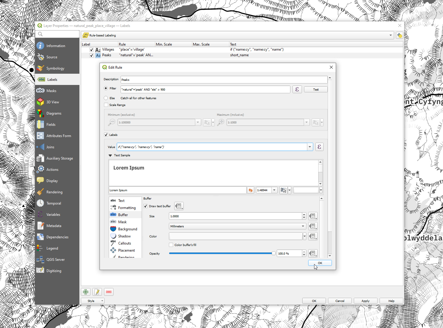
• Set the description to “Peaks”
• Set the filter to "natural"='peak' AND "ele" > 900
• Set the value to if ("name:cy", "name:cy", "name")
• Click on Text and set the font
• Set the text size to 10
• Click on Buffer and enable Draw text buffer
• Set the buffer size to 1
• Set the buffer colour to white
• Click on Placement and set the distance to -1

Click the Apply button and then close the symbology panel to see the result of all your hard work.

Taking things further

By now you should have a much deeper understanding of how to generate hachures in QGIS and also how to combine them with some basic monochrome cartography.

It’s completely up to you where to take things next, though here are some suggestions:

• Generating hill-shading to place under the hachures for extra detail
• Changing the contour generation settings to refine hachure density
• Tweaking the hachure styling to refine the balance of taper and opacity
• Adding different layers to the map to make it your own
• Optimising and automating this process even further

---

Share your creations on Twitter and make sure to tag me so I can see them.

I’d love to see versions of this in other locations, though I will never tire of maps of Eryri so I want to see those too!